Support Vector Machines in Python: Margins, Kernels, and C

Say you’ve split a dataset into two classes and drawn a straight line that puts every point on the correct side. Is the job done? Not really — there are usually many lines that separate two classes perfectly, and some of them pass so close to the data that a single new point could land on the wrong side of a boundary that only looked confident. K-Nearest Neighbors sidesteps that question entirely: it never draws a boundary at all, it just votes among nearby points at prediction time. Logistic regression draws exactly one boundary, wherever a fitted probability happens to cross 0.5, chosen by an optimization that never asks how close that line comes to the data it separates. A Support Vector Machine (SVM) asks a genuinely different question: of every line that separates the classes, which one has the most room to spare?

That’s an odd thing to optimize for the first time you meet it, and it’s easy to nod along without ever seeing why “most room to spare” beats “gets the training points right.” This post builds that idea first — the margin, and the small set of points called support vectors that actually decide where it sits — then works through a real dataset end to end: fitting a linear SVC, reading off its support vectors, tuning the C parameter, and reaching for the kernel trick when no straight line can do the job.

The Mental Model: The Widest Street Between Two Classes

Every other classifier on this site picks a boundary and stops there. An SVM keeps going:

1. Start from every line that separates the two classes perfectly. For most real datasets there isn’t just one — there’s a whole family of valid boundaries, all scoring 100% on the training data.
2. Measure each boundary’s margin — how far it sits from the nearest point of either class. Picture the boundary as the center line of a street; the margin is how wide you can make that street before a house on either side gets in the way.
3. Pick the boundary with the widest street. That’s the whole optimization: not “does it separate the classes,” which many lines do, but “how much breathing room does it leave.”
4. Only the closest houses matter. The points sitting exactly on the edge of that widest street are the support vectors. Every other point could be moved further from the boundary, or deleted outright, and the boundary wouldn’t shift a millimeter — it’s defined entirely by the handful of points closest to it.
5. Real data rarely separates perfectly, so a soft margin lets some points sit inside the street or even on the wrong side of it, in exchange for a wider, more stable boundary elsewhere. How much slack to allow is a dial, not a fact — that dial is the C parameter, covered later in this post.

The name makes more sense now: the vectors (points) that support (hold in place) the boundary are the only part of the training data the fitted model actually depends on.

A Dataset You Can Reproduce

This post uses the Wine Quality dataset: 1,599 red wines, each with eleven physicochemical lab measurements — acidity, sugar, chlorides, sulfur dioxide, density, pH, sulphates, and alcohol content — plus a quality score from 0 to 10 assigned by wine tasters. Imagine you run the lab for a small wine cooperative and want a quick, defensible screen for which barrels are likely to score well with the official tasting panel, using only measurements you already take in-house.

Data: the Wine Quality dataset (red wine subset), created by Cortez, Cerdeira, Almeida, Matos & Reis (2009) and hosted at the UCI Machine Learning Repository, licensed CC BY 4.0, vendored here as a plain CSV at /datasets/blog/support-vector-machines-in-python/winequality-red.csv.

import pandas as pd

wine = pd.read_csv(
    "https://datatweets.com/datasets/blog/support-vector-machines-in-python/winequality-red.csv",
    sep=";",
)
wine[["alcohol", "volatile acidity", "sulphates", "quality"]].head()

   alcohol  volatile acidity  sulphates  quality
0      9.4               0.70       0.56        5
1      9.8               0.88       0.68        5
2      9.8               0.76       0.65        5
3      9.8               0.28       0.58        6
4      9.4               0.70       0.56        5

wine.shape

(1599, 12)

wine["quality"].value_counts().sort_index()

quality
3     10
4     53
5    681
6    638
7    199
8     18
Name: count, dtype: int64

1,599 wines, eleven feature columns, and a quality score that’s almost never a 3 or an 8. That fine-grained scale is awkward to classify directly, so this post turns it into the yes/no question the lab actually cares about: is this wine good enough to send to the panel?

wine["good"] = (wine["quality"] >= 6).astype(int)
wine["good"].value_counts()

good
1    855
0    744
Name: count, dtype: int64

855 “good” wines (quality 6 and up) against 744 “not good” ones — close enough to balanced that plain accuracy is a fair headline metric for the rest of this post. (The outputs in this post come from pandas 3.0.3, numpy 2.4.6, and scikit-learn 1.9.0.)

One more check before modeling anything: which two features are worth plotting later, for a picture of the margin itself?

wine.drop(columns=["quality"]).corr(numeric_only=True)["good"].abs().sort_values(ascending=False)

good                    1.000
alcohol                 0.435
volatile acidity        0.321
total sulfur dioxide    0.232
sulphates               0.218
citric acid             0.159
density                 0.159
chlorides               0.109
fixed acidity           0.095
free sulfur dioxide     0.062
pH                      0.003
residual sugar          0.002
Name: good, dtype: float64

alcohol and volatile acidity are the two strongest single signals, so those are the pair this post comes back to for the 2D margin picture.

Fitting a Linear SVC

Set aside a test set the model never trains on — the same discipline every supervised model needs:

from sklearn.model_selection import train_test_split
from sklearn.svm import SVC
from sklearn.metrics import accuracy_score

X = wine.drop(columns=["quality", "good"])
y = wine["good"]
X_train, X_test, y_train, y_test = train_test_split(
    X, y, test_size=0.2, random_state=42, stratify=y
)
X_train.shape, X_test.shape

((1279, 11), (320, 11))

stratify=y keeps roughly the same 53/47 split of good in both slices. Now configure and fit a Support Vector Classifier with a linear kernel — a straight-line (or, with eleven features, flat-hyperplane) boundary:

svm = SVC(kernel="linear", random_state=42)
svm.fit(X_train, y_train)
y_pred = svm.predict(X_test)

acc_baseline = accuracy_score(y_test, y_pred)
print(f"accuracy (linear kernel, unscaled, all 11 features): {acc_baseline:.3f}")

accuracy (linear kernel, unscaled, all 11 features): 0.741

Same estimator shape as any other scikit-learn classifier — configure, .fit(), .predict(). What’s different is what’s sitting inside svm once it’s fitted, which is the whole point of the next section.

Identifying the Support Vectors

A fitted SVC remembers exactly which training rows ended up on the edge of its margin:

print("support_vectors_ shape:", svm.support_vectors_.shape)
print("n_support_ (per class):", svm.n_support_)
n_sv = svm.n_support_.sum()
print(f"{n_sv} of {len(X_train)} training rows are support vectors ({n_sv / len(X_train):.1%})")

support_vectors_ shape: (775, 11)
n_support_ (per class): [387 388]
775 of 1279 training rows are support vectors (60.6%)

775 of the 1,279 training wines — over 60% of them — are support vectors here. That’s a lot, and it’s a direct sign that “good” and “not good” wines overlap heavily across these eleven measurements rather than sitting in two clean clusters; a dataset with a wide, obvious gap between classes would leave far fewer points holding up the margin. The mental model’s claim is that these 775 rows are the entire fitted model — everything else is disposable. That’s testable:

X_sv = X_train.iloc[svm.support_]
y_sv = y_train.iloc[svm.support_]

svm_sv_only = SVC(kernel="linear", random_state=42)
svm_sv_only.fit(X_sv, y_sv)
y_pred_sv_only = svm_sv_only.predict(X_test)

print("predictions identical to the full-training-set model:", (y_pred_sv_only == y_pred).all())
print("rows dropped without changing a single prediction:", len(X_train) - n_sv)

predictions identical to the full-training-set model: True
rows dropped without changing a single prediction: 504

Refitting on only the 775 support vectors — throwing away 504 training rows entirely — produces the exact same predictions on the held-out test set. Every one of those 504 discarded rows sat far enough from the boundary that it had no say in where the margin landed in the first place.

Seeing the Margin in Two Dimensions

Eleven features are impossible to draw, but the two most correlated ones from earlier, alcohol and volatile acidity, fit on a page. Distance between points is about to matter for the boundary’s geometry, so this is also the first place features get scaled — more on why in the next section:

from sklearn.preprocessing import StandardScaler

X2 = wine[["alcohol", "volatile acidity"]]
X2_train, X2_test, y2_train, y2_test = train_test_split(
    X2, y, test_size=0.2, random_state=42, stratify=y
)
scaler2 = StandardScaler()
X2_train_s = scaler2.fit_transform(X2_train)
X2_test_s = scaler2.transform(X2_test)

svm2 = SVC(kernel="linear", C=1, random_state=42)
svm2.fit(X2_train_s, y2_train)
acc2 = accuracy_score(y2_test, svm2.predict(X2_test_s))
print(f"accuracy (2 features, scaled): {acc2:.3f}")
print(f"support vectors (2 features): {svm2.n_support_} = {svm2.n_support_.sum()} of {len(X2_train)}")

accuracy (2 features, scaled): 0.753
support vectors (2 features): [413 414] = 827 of 1279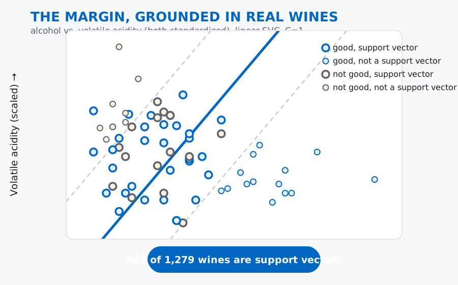

With only two of the eleven features to work with, 827 of the 1,279 training wines — nearly two-thirds — turn out to be support vectors, even more than the full-feature model’s 775. The diagram shows why: on just alcohol and volatile acidity, good and not-good wines genuinely overlap around the boundary instead of splitting into two obvious clouds, so a wide band of points ends up sitting inside or right on the margin. That’s not a bug in the fit — it’s an honest picture of how separable these two measurements really are on their own; the other nine features in the full model are doing real work narrowing that overlap down.

Why Feature Scaling Matters for SVMs, Too

Like K-Nearest Neighbors, an SVM’s boundary is ultimately a distance calculation, so it inherits the same sensitivity to feature scale. Refit the full eleven-feature linear model on standardized data and compare:

scaler = StandardScaler()
X_train_s = scaler.fit_transform(X_train)
X_test_s = scaler.transform(X_test)

svm_linear_scaled = SVC(kernel="linear", random_state=42)
svm_linear_scaled.fit(X_train_s, y_train)
acc_linear_scaled = accuracy_score(y_test, svm_linear_scaled.predict(X_test_s))

print(f"accuracy (linear kernel, unscaled): {acc_baseline:.3f}")
print(f"accuracy (linear kernel, scaled):   {acc_linear_scaled:.3f}")

accuracy (linear kernel, unscaled): 0.741
accuracy (linear kernel, scaled):   0.744

A small gain for the linear kernel here — keep that number in mind, because the kernel trick section below shows scaling matters far more once the boundary stops being a straight line. The reason scaling matters at all is the same one KNN ran into, just applied to a different pair of columns this time:

stds = X_train[["total sulfur dioxide", "chlorides"]].std()
print(stds.round(3))

r1, r2 = X_train.iloc[0], X_train.iloc[1]
d_so2 = (r1["total sulfur dioxide"] - r2["total sulfur dioxide"]) ** 2
d_chl = (r1["chlorides"] - r2["chlorides"]) ** 2
share = d_so2 / (d_so2 + d_chl) * 100
print(f"squared difference in total sulfur dioxide: {d_so2:.2f}")
print(f"squared difference in chlorides: {d_chl:.6f}")
print(f"total sulfur dioxide alone accounts for {share:.4f}% of their combined squared distance")

total sulfur dioxide    33.193
chlorides                 0.046
dtype: float64
squared difference in total sulfur dioxide: 64.00
squared difference in chlorides: 0.000036
total sulfur dioxide alone accounts for 99.9999% of their combined squared distance

total sulfur dioxide is measured in parts per million and swings across dozens of units between wines; chlorides is a small fraction of a gram and barely moves. Left unscaled, total sulfur dioxide alone decides almost the entire distance between these two wines, and chlorides — genuinely relevant to a taster — contributes essentially nothing to where the margin gets drawn.

The C Parameter: Margin Width vs. Misclassification Tolerance

C is the soft-margin dial from the mental model: how much a wrongly-placed or margin-violating point should cost the optimizer. A small C says “a wide, calm margin matters more than a few mistakes”; a large C says “push the margin in wherever it takes to get more points on the right side.” Sweep it on the scaled, full-feature data:

for C in [0.01, 1, 100]:
    m = SVC(kernel="linear", C=C, random_state=42)
    m.fit(X_train_s, y_train)
    acc = accuracy_score(y_test, m.predict(X_test_s))
    print(f"C={C:>6}: accuracy={acc:.3f}  support_vectors={m.n_support_.sum()}")

C=  0.01: accuracy=0.731  support_vectors=853
C=     1: accuracy=0.744  support_vectors=763
C=   100: accuracy=0.738  support_vectors=763

At C=0.01, the optimizer barely penalizes margin violations, so the margin stays wide and loose — more points (853) end up inside it, and accuracy is the lowest of the three. At C=1, tightening the penalty narrows the margin, drops the support-vector count to 763, and buys the best accuracy of the sweep. Push further to C=100 and the support-vector count doesn’t move at all (still 763) — the solver has already converged on essentially the same boundary — but accuracy dips slightly to 0.738, a small sign of overfitting to a few borderline training points that don’t generalize. Bigger C isn’t automatically better; it’s a real tradeoff, which is exactly why the gotchas section below argues for validating it rather than guessing.

The Kernel Trick: When a Straight Line Isn’t Enough

Every boundary so far has been flat — a straight line in 2D, a flat hyperplane in 11D. SVC’s kernel argument can bend that boundary into a curve without you ever having to invent new features by hand. A rbf (radial basis function) kernel measures how similar two points are based on their distance, and lets the fitted boundary curve around clusters instead of cutting straight through them. Full details on every kernel option live in scikit-learn’s SVC reference.

svm_rbf_unscaled = SVC(kernel="rbf", random_state=42)
svm_rbf_unscaled.fit(X_train, y_train)
acc_rbf_unscaled = accuracy_score(y_test, svm_rbf_unscaled.predict(X_test))

svm_rbf_scaled = SVC(kernel="rbf", random_state=42)
svm_rbf_scaled.fit(X_train_s, y_train)
acc_rbf_scaled = accuracy_score(y_test, svm_rbf_scaled.predict(X_test_s))

print(f"rbf kernel, unscaled:  {acc_rbf_unscaled:.3f}")
print(f"linear kernel, scaled: {acc_linear_scaled:.3f}")
print(f"rbf kernel, scaled:    {acc_rbf_scaled:.3f}")

rbf kernel, unscaled:  0.647
linear kernel, scaled: 0.744
rbf kernel, scaled:    0.762

Two things are happening in that short table. First, rbf on unscaled data (0.647) is actually worse than the unscaled linear kernel from earlier (0.741) — because rbf’s similarity measure is a raw distance calculation, it’s even more exposed to the scale problem from the previous section than the linear kernel’s dot product is. Second, once features are scaled fairly, rbf (0.762) pulls ahead of linear (0.744). That gap is real evidence of non-linear structure: eleven physicochemical measurements don’t separate good wine from not-good wine along a flat boundary, and letting the kernel curve gains a few points of accuracy a straight line simply can’t reach.

Four Gotchas Worth Knowing

Forgetting to scale hurts rbf far more than it hurts linear. Both kernels improved with scaling, but not by the same amount:

print(f"linear kernel: unscaled={acc_baseline:.3f}  scaled={acc_linear_scaled:.3f}  (+{acc_linear_scaled - acc_baseline:.3f})")
print(f"rbf kernel:    unscaled={acc_rbf_unscaled:.3f}  scaled={acc_rbf_scaled:.3f}  (+{acc_rbf_scaled - acc_rbf_unscaled:.3f})")

linear kernel: unscaled=0.741  scaled=0.744  (+0.003)
rbf kernel:    unscaled=0.647  scaled=0.762  (+0.116)

Linear gained three-tenths of a point from scaling; rbf gained nearly twelve. If you only ever test the linear kernel unscaled, scaling can look optional — the moment you reach for rbf, it stops being optional at all.

Picking C and the kernel by eyeballing the test set is how you quietly overfit your own evaluation. Every comparison above touched the test set repeatedly to explain a concept — for a real project, that’s exactly what a held-out validation split, carved from the training data alone, is for:

X_train_sub, X_val, y_train_sub, y_val = train_test_split(
    X_train_s, y_train, test_size=0.25, random_state=42, stratify=y_train
)

best_acc, best_kernel, best_C = 0, None, None
for kernel in ["linear", "rbf"]:
    for C in [0.1, 1, 10]:
        m = SVC(kernel=kernel, C=C, random_state=42)
        m.fit(X_train_sub, y_train_sub)
        acc = accuracy_score(y_val, m.predict(X_val))
        print(f"kernel={kernel:<6} C={C:>4}: validation accuracy={acc:.4f}")
        if acc > best_acc:
            best_acc, best_kernel, best_C = acc, kernel, C

print(f"best on validation: kernel={best_kernel}, C={best_C} (accuracy={best_acc:.4f})")

kernel=linear C= 0.1: validation accuracy=0.7063
kernel=linear C=   1: validation accuracy=0.7094
kernel=linear C=  10: validation accuracy=0.7094
kernel=rbf    C= 0.1: validation accuracy=0.7406
kernel=rbf    C=   1: validation accuracy=0.7406
kernel=rbf    C=  10: validation accuracy=0.7438
best on validation: kernel=rbf, C=10 (accuracy=0.7438)

final_svm = SVC(kernel=best_kernel, C=best_C, random_state=42)
final_svm.fit(X_train_s, y_train)
final_acc = accuracy_score(y_test, final_svm.predict(X_test_s))
print(f"held-out test accuracy with kernel={best_kernel}, C={best_C}: {final_acc:.3f}")

held-out test accuracy with kernel=rbf, C=10: 0.772

rbf with C=10 won on the validation split the test set never touched, and that choice happens to beat every combination tried earlier in this post on the real held-out test set too (0.772). The point isn’t that C=10 is universally correct — it’s that this number came from a systematic check instead of a guess.

Training an SVC gets slow, non-linearly, as the training set grows. Fitting time isn’t roughly constant the way LogisticRegression’s is — it grows faster than the data does:

import time
import numpy as np

rng = np.random.default_rng(0)
for n in [500, 2000, 8000]:
    Xt = rng.normal(size=(n, 11))
    yt = rng.integers(0, 2, size=n)
    t0 = time.perf_counter()
    SVC(kernel="rbf").fit(Xt, yt)
    dt = time.perf_counter() - t0
    print(f"n_train={n:>6,}: SVC(kernel='rbf').fit() took {dt * 1000:7.1f}ms")

n_train=   500: SVC(kernel='rbf').fit() took     5.6ms
n_train= 2,000: SVC(kernel='rbf').fit() took    86.0ms
n_train= 8,000: SVC(kernel='rbf').fit() took  1423.6ms

Training rows grew 4x twice in a row (500 to 2,000, then 2,000 to 8,000), but fit time grew roughly 15x each time — nowhere near proportional. This dataset’s 1,279 training rows are small enough that it’s invisible; scikit-learn’s own documentation notes SVC training scales worse than linearly and becomes impractical somewhere past tens of thousands of rows, which is worth knowing before reaching for an SVM on a genuinely large dataset.

A linear kernel doesn’t error or warn when the data genuinely isn’t linearly separable — it just quietly underperforms. The kernel trick section above found a real gap between linear (0.744) and rbf (0.762) on the exact same scaled data, and nothing about fitting the weaker model looked wrong from the inside:

import warnings

with warnings.catch_warnings(record=True) as caught:
    warnings.simplefilter("always")
    SVC(kernel="linear", random_state=42).fit(X_train_s, y_train)
    print("warnings raised while fitting the linear kernel on non-linearly-separable data:", len(caught))

warnings raised while fitting the linear kernel on non-linearly-separable data: 0

Zero warnings, a clean fit, a perfectly plausible-looking accuracy number — SVC(kernel="linear") will happily hand you a working model on data it can’t actually separate well, with nothing in the output flagging that a curved boundary would have done better. The only way to catch it is the same fix as the C gotcha above: compare kernels on a validation split instead of assuming linear is good enough.

Wrapping Up

One mental model covers the whole algorithm: find the boundary with the widest margin, let the support vectors closest to it define where it sits, and use C and the kernel to control how that boundary bends and how much slack it tolerates. Mapped onto the tools:

• Maximum margin → among every boundary that separates the classes, SVC picks the one furthest from the nearest point of each
• .support_vectors_ / .n_support_ → the only training rows the fitted boundary actually depends on
• C → small values tolerate more margin violations for a wider, calmer boundary; large values tighten the margin at the risk of overfitting a few borderline points
• kernel="rbf" → bends the boundary to fit data a straight line can’t separate, at the cost of being even more sensitive to unscaled features
• StandardScaler → essential before fitting either kernel, and especially before rbf

If you want the guided version of classification fundamentals that this post builds on — logistic regression, evaluation metrics, and a full guided project — the Classification module in our free Machine Learning course is the natural next stop, and the K-Nearest Neighbors deep dive covers the other end of the “how is the boundary chosen” spectrum this post opened with.