The same neural-network settings produced sharply different validation scores in this lesson. Seed 19 reached 0.505 balanced accuracy, while seed 11 reached 0.608, even though both runs used the same rows, features, and settings. A report containing only seed 11 would hide that variation.

To test neural network stability across random seeds, freeze the data split and preprocessing, fit a fresh copy of the same model configuration with each of several explicit random_state values, and record both metric variation and per-row probability variation. Report the minimum, mean, maximum, and standard deviation across runs; do not treat the seed with the highest score as a model setting.

We will apply that procedure to a fictional data-import review system. The model estimates whether a new CSV import needs manual review. This is a controlled teaching example, not an automated rule for accepting real data.

Setup, prerequisites, and teaching data

You need Python 3.11 or newer. You should know basic Python variables and pandas tables. You also need to know that a classifier assigns a row to a category. If model fitting and test data are new ideas, begin with How to Build Your First Machine Learning Model.

Create and activate a virtual environment, then install the four packages used by the executed build:

python -m venv .venv
source .venv/bin/activate
python -m pip install numpy pandas scikit-learn matplotlib

On Windows PowerShell, activate it with .venv\Scripts\Activate.ps1. The published run used Python 3.13.2, NumPy 2.5.1, pandas 3.0.3, scikit-learn 1.9.0, and Matplotlib 3.11.0.

Download data_import_batches.csv and save it beside your Python file or notebook. This original synthetic dataset was generated with NumPy seed 20260722 and is released under CC0-1.0. Synthetic means code created the rows. All batch IDs, quality measurements, and review labels are fictional.

Load the file and inspect three rows before modeling. This small check reveals the column names, units, table size, and class counts:

import pandas as pd

imports = pd.read_csv("data_import_batches.csv")
print(imports.shape)
print(imports.head(3).to_string(index=False))
print(imports["needs_manual_review"].value_counts().sort_index())

(1200, 10)
   batch_id  rows_received  columns_detected  missing_cell_pct  duplicate_row_pct  parse_error_pct  mixed_type_columns  encoding_warnings  source_age_days  needs_manual_review
IMPORT-0001         170058                37              6.89               3.60             0.02                   1                  0              104                    0
IMPORT-0002         468162                65              1.30               0.09             0.39                   3                  0               28                    0
IMPORT-0003          92008                15              4.06               0.82             0.57                   0                  1              162                    0
needs_manual_review
0    832
1    368

There are 1,200 batches. Eight numeric feature columns describe file size, shape, missing cells, duplicates, parsing problems, mixed data types, encoding warnings, and source age. The target is needs_manual_review: 1 means review and 0 means no review. About 31% of rows have label 1, so plain accuracy could give too much influence to the larger class.

Understanding what one seed controls

A random seed is an integer that starts a repeatable sequence of pseudorandom choices. An algorithm produces these choices. They look random, but the same code, data, software versions, and integer can reproduce the sequence.

Neural-network training needs such choices. The starting weights are initialized before learning. The Adam solver also trains with small shuffled batches rather than the complete table at once. With early stopping enabled, scikit-learn reserves an internal validation sample from the supplied training rows.

The current MLPClassifier documentation states that random_state controls weight and bias initialization, the early-stopping split, and batch sampling for Adam or stochastic gradient descent. Changing the integer can therefore lead training through a different path.

This does not mean the model is defective. One seeded fit is one possible outcome of the training procedure. A useful stability audit separates two kinds of variation:

fixed in this audit                 changed in this audit
-------------------                 ---------------------
dataset rows                        model random_state
train/validation/test split
feature scaling
network shape and training settings
metric definitions

If you change the split and model seed together, you cannot tell whether a score changed because of different data or different training choices. Both questions matter, but they need separate experiments. This lesson measures training variation first.

An integer seed gives repeatability. It does not prove stability. A model can reproduce one unusually strong or weak outcome perfectly.

Freeze the outer data split

Use one fixed, stratified split for all twelve runs. Stratified means each part keeps approximately the same class proportions. We will assign 40% of the data to training, 30% to validation, and 30% to final testing:

from sklearn.model_selection import train_test_split

feature_columns = [
    "rows_received",
    "columns_detected",
    "missing_cell_pct",
    "duplicate_row_pct",
    "parse_error_pct",
    "mixed_type_columns",
    "encoding_warnings",
    "source_age_days",
]

X = imports[feature_columns]
y = imports["needs_manual_review"]

X_train, X_later, y_train, y_later = train_test_split(
    X,
    y,
    train_size=0.40,
    stratify=y,
    random_state=41027,
)
X_validation, X_test, y_validation, y_test = train_test_split(
    X_later,
    y_later,
    test_size=0.50,
    stratify=y_later,
    random_state=41027,
)

print(len(X_train), len(X_validation), len(X_test))

480 360 360

The 480 training rows update model weights. The 360 validation rows measure seed-to-seed variation. The 360 test rows remain unused until the audit procedure and comparison methods are fixed.

The small training set is intentional. It makes variation easy to observe in a quick CPU lesson. A larger representative dataset may reduce variation, but size alone does not guarantee stability.

Build one model recipe, then supply a seed

The input columns use very different scales. rows_received can be in the hundreds of thousands, while parse_error_pct is usually a small number. StandardScaler centers each feature and scales its variation. A scikit-learn Pipeline fits the scaler only on training rows and applies the stored transformation during validation and testing.

The official pipeline guide recommends this structure because it keeps preprocessing with the estimator and helps prevent test statistics from entering training.

Define a function that accepts one seed. Every other setting stays constant:

from sklearn.neural_network import MLPClassifier
from sklearn.pipeline import Pipeline
from sklearn.preprocessing import StandardScaler

def make_model(seed):
    return Pipeline([
        ("scale", StandardScaler()),
        ("network", MLPClassifier(
            hidden_layer_sizes=(24, 12),
            activation="relu",
            solver="adam",
            alpha=0.002,
            batch_size=32,
            learning_rate_init=0.002,
            max_iter=350,
            early_stopping=True,
            validation_fraction=0.18,
            n_iter_no_change=18,
            random_state=seed,
        )),
    ])

The two hidden layers contain 24 and 12 units, also called neurons. alpha adds a penalty for large weights. Early stopping ends training after the internal validation score fails to improve enough for 18 epochs. These values are fixed lesson choices, not recommended settings for every dataset.

Notice that the internal early-stopping sample comes only from X_train. It is separate from our 360-row outer validation set. The outer set gives every completed run the same comparison data.

Run the seed audit and summarize the distribution

We need metrics that show different behavior. Balanced accuracy averages recall across both classes, giving manual-review and no-review rows equal weight. Higher is better. Log loss measures predicted probabilities and penalizes confident wrong answers. Lower is better.

The current scikit-learn references define balanced accuracy as average class recall and log loss as probability-based cross-entropy loss.

Fit one fresh pipeline per integer. Save the probability vector as well as the run-level metrics. Creating a new pipeline makes each run independent and prevents state from carrying over if you later enable options such as warm_start:

import numpy as np
from sklearn.metrics import balanced_accuracy_score, log_loss

seeds = [3, 7, 11, 19, 23, 31, 43, 47, 59, 61, 73, 89]
run_rows = []
validation_probabilities = []
models = []

for seed in seeds:
    model = make_model(seed)
    model.fit(X_train, y_train)
    probability = model.predict_proba(X_validation)[:, 1]
    prediction = (probability >= 0.5).astype(int)

    run_rows.append({
        "seed": seed,
        "epochs": model.named_steps["network"].n_iter_,
        "validation_balanced_accuracy": balanced_accuracy_score(
            y_validation, prediction
        ),
        "validation_log_loss": log_loss(y_validation, probability),
    })
    validation_probabilities.append(probability)
    models.append(model)

runs = pd.DataFrame(run_rows)
print(runs.round(3).to_string(index=False))

 seed  epochs  validation_balanced_accuracy  validation_log_loss
    3      46                         0.575                0.589
    7      24                         0.549                0.602
   11      30                         0.608                0.582
   19      22                         0.505                0.604
   23      31                         0.516                0.596
   31      41                         0.570                0.572
   43      45                         0.590                0.592
   47      36                         0.606                0.559
   59      32                         0.582                0.569
   61      24                         0.505                0.609
   73      27                         0.554                0.581
   89      28                         0.570                0.573

The complete executed table is available as seed_run_metrics.csv.

Now summarize balanced accuracy across runs. Use sample standard deviation, written as std(ddof=1), to describe how much the twelve observed scores vary around their mean:

score = runs["validation_balanced_accuracy"]
print(f"minimum: {score.min():.3f}")
print(f"mean:    {score.mean():.3f}")
print(f"maximum: {score.max():.3f}")
print(f"std:     {score.std(ddof=1):.3f}")

minimum: 0.505
mean:    0.561
maximum: 0.608
std:     0.036

The 0.103 gap between minimum and maximum is large relative to the mean. In this audit, the model configuration is sensitive to training randomness on the given 480 rows. The mean describes these twelve runs better than the maximum does, but it is not a promise for new data.

Do not tune random_state by keeping seed 11 because it has the highest balanced accuracy. A seed does not describe a meaningful property of future import batches. Choosing it after reading validation results turns random variation into hidden model selection.

Find rows whose decisions change

An average metric can hide local disagreement. Stack the twelve probability arrays into a matrix. Each row of this matrix represents a model seed, and each column represents one validation batch:

probability_matrix = np.vstack(validation_probabilities)
label_matrix = (probability_matrix >= 0.5).astype(int)

changed_label = label_matrix.min(axis=0) != label_matrix.max(axis=0)
print(f"changed labels: {changed_label.sum()} / {len(y_validation)}")

changed labels: 124 / 360

For 124 validation batches, at least one model predicted manual review and at least one predicted no review. That is more operationally concrete than the score standard deviation: about one-third of the rows did not receive a consistent class across these twelve runs.

The next calculation finds rows with the widest probability range. It reports the minimum, mean, and maximum probability plus the number of models that crossed the 0.50 review cutoff:

details = pd.DataFrame({
    "batch_id": imports.loc[X_validation.index, "batch_id"].to_numpy(),
    "actual_review": y_validation.to_numpy(),
    "minimum_probability": probability_matrix.min(axis=0),
    "mean_probability": probability_matrix.mean(axis=0),
    "maximum_probability": probability_matrix.max(axis=0),
    "review_votes_out_of_12": label_matrix.sum(axis=0),
})
details["probability_range"] = (
    details["maximum_probability"] - details["minimum_probability"]
)

shown = details.nlargest(4, "probability_range")
print(shown.drop(columns="probability_range").round(3).to_string(index=False))

   batch_id  actual_review  minimum_probability  mean_probability  maximum_probability  review_votes_out_of_12
IMPORT-0770              1                0.270             0.499                0.809                       4
IMPORT-0367              1                0.196             0.440                0.719                       5
IMPORT-0923              0                0.123             0.347                0.645                       2
IMPORT-0702              0                0.286             0.519                0.790                       7

For IMPORT-0770, probabilities range from 0.270 to 0.809. Only 4 of 12 models cross the review cutoff, even though the mean probability is almost exactly 0.5. Reporting one seed would conceal this disagreement.

The generated chart combines the run-level and row-level views:

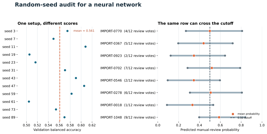
Read the left panel vertically: every dot is the same recipe with a different seed, and the orange line is the mean. In the right panel, each gray segment spans the smallest to largest probability assigned to one batch. Crossing the dashed 0.50 line means the final label depends on the seed.

You can inspect all eight displayed rows in seed_disagreement_examples.csv. These rows are candidates for error analysis. They may reveal limited training coverage, overlapping classes, weak features, noisy labels, or a decision cutoff that needs separate evaluation.

Check a predefined ensemble without promising an improvement

One way to combine repeated models is a probability ensemble: average their class-1 probabilities, then apply the decision cutoff once. We will compare that predefined method with seed 3, the first seed in the list. Neither choice is based on the validation winner.

Only now generate probabilities for the untouched test rows:

test_probability_matrix = np.vstack([
    model.predict_proba(X_test)[:, 1] for model in models
])

seed_3_probability = test_probability_matrix[0]
ensemble_probability = test_probability_matrix.mean(axis=0)

seed_3_prediction = (seed_3_probability >= 0.5).astype(int)
ensemble_prediction = (ensemble_probability >= 0.5).astype(int)

print(
    "seed 3 balanced accuracy:",
    round(balanced_accuracy_score(y_test, seed_3_prediction), 3),
)
print(
    "ensemble balanced accuracy:",
    round(balanced_accuracy_score(y_test, ensemble_prediction), 3),
)
print("seed 3 log loss:", round(log_loss(y_test, seed_3_probability), 3))
print("ensemble log loss:", round(log_loss(y_test, ensemble_probability), 3))

seed 3 balanced accuracy: 0.605
ensemble balanced accuracy: 0.573
seed 3 log loss: 0.583
ensemble log loss: 0.578

The ensemble has slightly lower log loss, so it scored better on this test set under that metric. Its balanced accuracy is lower because averaging changes which probabilities sit above 0.50. This is why “use an ensemble” is not a complete conclusion. Evaluate the metric tied to the real decision, and do not assume averaging improves every measure.

These scores also do not make the synthetic classifier suitable for real import approval. A real system needs representative files, reviewed labels, subgroup checks, cost-based thresholds, monitoring, and a manual fallback.

Common mistakes and troubleshooting

Changing the data split for every model seed. This mixes sampling variation with training variation. Keep the outer split fixed for this audit. Run a separate repeated-split or cross-validation study when you want both sources of uncertainty.

Reporting only the best seed. The largest score is an extreme from the measured distribution. Report the seed list, all run metrics, and a summary. Treat the seed as an experimental control, not a hyperparameter to optimize.

Leaving random_state=None. Repeated fits may differ, but the exact experiment cannot be reproduced. Use an explicit list of integers and store it with the results. Scikit-learn’s randomness guidance explains the difference between integers, RandomState instances, and None.

Fitting the scaler before splitting. A scaler fitted on all rows learns validation and test statistics. Split first and keep StandardScaler inside the pipeline.

Reusing a warm-started model. With warm_start=True, a later call to fit() can reuse the previous solution instead of starting an independent run. Construct a fresh pipeline inside the loop.

Comparing rounded probabilities. Calculate labels and metrics from full-precision arrays. Round only the printed table. A displayed 0.500 may be slightly above or below the cutoff internally.

Measuring only a single score. Balanced accuracy describes class decisions, while log loss describes probability quality. Add row-level ranges to find cases where operational labels change.

Assuming a small standard deviation proves safety. Stable models can be consistently wrong because of biased data, leakage, label errors, or distribution shift. Stability is one diagnostic, not complete validation.

Expecting exact numbers with different versions. Integer seeds make the tested environment repeatable, but numerical libraries and implementation details can change. Record Python and package versions with serious experiments.

Recap: a small audit before trusting one result

A fixed seed answers “Can I reproduce this run?” A seed audit answers the more useful question: “Does the training procedure behave similarly when its random choices change?”

For this synthetic import-review model, twelve runs produced validation balanced accuracy from 0.505 to 0.608, with a mean of 0.561 and a sample standard deviation of 0.036. Predicted labels differed across runs on 124 of 360 validation rows. The probability ensemble slightly reduced test log loss but also reduced test balanced accuracy, so it was not a universal improvement.

Keep this short audit for your next stochastic model:

1. Freeze the data split, preprocessing, settings, and metrics.
2. Fit fresh models with a recorded list of seeds.
3. Save every score and prediction probability.
4. Report the score distribution, not only its maximum.
5. Count rows whose labels or probabilities change materially.
6. Evaluate any response, such as averaging, against untouched data and the metric that matches the decision.

The next useful experiment is a separate repeated-split audit. Keep the model-seed list fixed, vary the outer split seed, and compare variation between splits with variation between training runs. That shows whether the larger uncertainty comes from which rows were sampled or how the network learned from them.