How to Test a Python Time Series Forecasting Environment

A forecasting script can import every package and still fail when the parts meet. Dates may be out of order, a validation split may train on future rows, a model may not fit, or a plotting backend may require a desktop window. Finding one of these problems after a long experiment wastes time.

To test a Python time series forecasting environment, create an isolated virtual environment and run one small script that loads dated data, makes ordered train-test folds, fits a model, calculates an error metric, and saves a chart. The setup is ready only when that complete path finishes with sensible dates, finite scores, and a real image file.

This tutorial builds that smoke test, which is a quick check that the main parts work together. It is not a search for the best forecast. We will use a small synthetic series so installation and integration problems are easier to see than they would be in a large project.

Prerequisites and Setup for an Isolated Project

You need Python 3 and a terminal where you can run commands. You do not need forecasting experience. Basic Python syntax is helpful, but each time-series term is defined before it is used.

Start in an empty project folder. Create a virtual environment, an isolated directory that holds this project’s Python interpreter and packages:

python -m venv .venv
source .venv/bin/activate

On Windows PowerShell, use .venv\Scripts\Activate.ps1 for the second command. Python’s current venv documentation explains that environments keep their own package set and are meant to be recreated rather than moved between folders.

Create a file named requirements.txt with the tested package versions:

numpy==2.5.1
pandas==3.0.3
scikit-learn==1.9.0
statsmodels==0.14.6
matplotlib==3.11.0

Install those packages through the active interpreter:

python -m pip install -r requirements.txt

Using python -m pip makes the interpreter choice visible. The Python Packaging User Guide documents the same requirements.txt installation command. Exact pins make this lesson’s output easier to reproduce. For a maintained application, update dependencies in a separate branch, rerun tests, and record the new working set instead of keeping old versions forever.

The published run used Python 3.13.2 and the five package versions above.

How a Forecasting Smoke Test Works

An import check answers only one question: can Python find this package? A useful integration check goes through five layers:

1. Interpreter: the script is running inside a virtual environment and reports the versions it uses.
2. Data: pandas can parse, sort, and validate a complete daily time index.
3. Evaluation: scikit-learn can create test periods that occur after their training periods.
4. Forecast: statsmodels can fit and forecast without producing missing or infinite values.
5. Output: Matplotlib can save a chart without a graphical desktop.

The test data represents daily sample arrivals at a fictional laboratory. Download lab_sample_arrivals.csv and save it beside your Python file. The 196 dates and counts were generated with a fixed NumPy random seed for this lesson. They do not describe a real laboratory. The dataset is released under CC0-1.0, so you may reuse it without restriction.

The generated series has a gentle rise, a repeating weekday pattern, and random variation. Its purpose is to make a seven-day forecasting path run, not to imitate a particular organization.

Confirm the Interpreter and Package Versions

Create forecast_smoke_test.py. The first part selects Matplotlib’s non-interactive Agg backend before importing pyplot. This order matters on servers and automated jobs where no screen is available. It also imports Path, which the final check uses to inspect the saved SVG file.

import platform
import sys
from pathlib import Path

import matplotlib

matplotlib.use("Agg")

import matplotlib.pyplot as plt
import numpy as np
import pandas as pd
import sklearn
import statsmodels
from sklearn.metrics import mean_absolute_error
from sklearn.model_selection import TimeSeriesSplit
from statsmodels.tsa.holtwinters import ExponentialSmoothing

print("isolated environment:", sys.prefix != sys.base_prefix)
print("python:", platform.python_version())
print("numpy:", np.__version__)
print("pandas:", pd.__version__)
print("scikit-learn:", sklearn.__version__)
print("statsmodels:", statsmodels.__version__)
print("matplotlib:", matplotlib.__version__)

The sys.prefix comparison is the check recommended by the official venv documentation. It should print True when the script runs inside a virtual environment. This test does not identify a specific environment, so the version lines help confirm that you activated the one you intended:

isolated environment: True
python: 3.13.2
numpy: 2.5.1
pandas: 3.0.3
scikit-learn: 1.9.0
statsmodels: 0.14.6
matplotlib: 3.11.0

Versions alone do not say that these libraries can exchange data correctly. They provide a useful diagnostic record when another computer produces a different result.

Make the Timeline Fail Clearly

Now load the CSV, parse date as a datetime value, sort it, and make it the row index. A DatetimeIndex is a pandas index that understands calendar dates.

samples = pd.read_csv(
    "lab_sample_arrivals.csv",
    parse_dates=["date"],
)
samples = samples.sort_values("date").set_index("date")

if samples.index.duplicated().any():
    raise ValueError("Duplicate dates found")
if pd.infer_freq(samples.index) != "D":
    raise ValueError("Dates are not one complete daily sequence")
if samples["samples_received"].isna().any():
    raise ValueError("Missing target values found")

series = samples["samples_received"].asfreq("D")
print(series.head(8).to_string())

The current pandas infer_freq documentation says the function returns the most likely spacing of a datetime-like sequence. D means one row per calendar day.

date
2025-01-06    53
2025-01-07    50
2025-01-08    48
2025-01-09    44
2025-01-10    44
2025-01-11    30
2025-01-12    29
2025-01-13    54
Freq: D

The first eight values make the weekly shape visible: arrivals fall over the weekend and rise again on Monday. More importantly, the checks stop the script before modeling if a date is duplicated, a day is absent, or a target is missing.

Do not automatically replace a missing daily count with zero. Zero means the laboratory observed no samples. A missing value means the count is unknown. Those facts need different handling.

Create Future-Only Test Folds

A fold is one training set paired with one test set. Normal random cross-validation can train on later dates and test on earlier ones. That gives a forecasting model information from its future.

Use TimeSeriesSplit to create three expanding training sets. Each test covers the next 14 days:

splitter = TimeSeriesSplit(n_splits=3, test_size=14)

for fold, (train_positions, test_positions) in enumerate(
    splitter.split(series), start=1
):
    train = series.iloc[train_positions]
    test = series.iloc[test_positions]

    assert train.index.max() < test.index.min()
    print(
        f"fold {fold}: train {train.index.min().date()} to "
        f"{train.index.max().date()} ({len(train)} rows); "
        f"test {test.index.min().date()} to "
        f"{test.index.max().date()} ({len(test)} rows)"
    )

fold 1: train 2025-01-06 to 2025-06-08 (154 rows); test 2025-06-09 to 2025-06-22 (14 rows)
fold 2: train 2025-01-06 to 2025-06-22 (168 rows); test 2025-06-23 to 2025-07-06 (14 rows)
fold 3: train 2025-01-06 to 2025-07-06 (182 rows); test 2025-07-07 to 2025-07-20 (14 rows)

Read each line from left to right. The training end is always earlier than the test start. The training history grows by 14 rows after each fold, while every test remains 14 days long.

The official scikit-learn TimeSeriesSplit documentation notes that its later training sets contain the earlier ones and that equally spaced samples are needed for comparable fold durations. Our earlier D check confirms that spacing.

Exercise a Real Forecast and a Baseline

The model check uses additive Holt-Winters exponential smoothing. Additive means the estimated level, upward trend, and weekday adjustment are combined in the same sample-count units. seasonal_periods=7 tells the model that one daily cycle contains seven observations.

A smoke test also needs a simple reference. The seasonal-naive baseline repeats the final known week. If the last training period ended on Sunday, its first test prediction copies the previous Monday, its second copies the previous Tuesday, and so on. For a full lesson about that method, see how to build and backtest a seasonal naive forecast.

Add a helper that repeats the seven known values for a 14-day test:

def repeat_last_week(train, steps):
    return np.resize(train.iloc[-7:].to_numpy(), steps)

Next, rebuild the splitter and fit both methods inside each fold. Mean absolute error (MAE) is the average absolute distance between actual and predicted values. It stays in samples, and lower is better. The explicit checks make a wrong fold, wrong forecast length, or non-finite prediction stop the smoke test immediately.

rows = []
final_predictions = None

for fold, (train_positions, test_positions) in enumerate(
    splitter.split(series), start=1
):
    train = series.iloc[train_positions]
    test = series.iloc[test_positions]

    if train.index.max() >= test.index.min():
        raise AssertionError("A fold trains on its future")
    if len(test) != 14:
        raise AssertionError("Unexpected test length")

    model = ExponentialSmoothing(
        train,
        trend="add",
        seasonal="add",
        seasonal_periods=7,
        initialization_method="estimated",
    ).fit(optimized=True)

    model_forecast = model.forecast(len(test))
    naive_forecast = repeat_last_week(train, len(test))

    if len(model_forecast) != len(test):
        raise AssertionError("Unexpected forecast length")
    if not np.isfinite(model_forecast.to_numpy()).all():
        raise ValueError("Holt-Winters returned a non-finite forecast")
    if not np.isfinite(naive_forecast).all():
        raise ValueError("Seasonal naive returned a non-finite forecast")

    rows.append({
        "fold": fold,
        "holt_winters_mae": round(
            float(mean_absolute_error(test, model_forecast)), 2
        ),
        "seasonal_naive_mae": round(
            float(mean_absolute_error(test, naive_forecast)), 2
        ),
    })

    if fold == 3:
        final_predictions = pd.DataFrame({
            "actual": test,
            "holt_winters": model_forecast,
            "seasonal_naive": naive_forecast,
        })

scores = pd.DataFrame(rows)
print(scores.to_string(index=False))
print(f"\nmean Holt-Winters MAE: {scores['holt_winters_mae'].mean():.2f}")
print(
    "mean seasonal-naive MAE: "
    f"{scores['seasonal_naive_mae'].mean():.2f}"
)

Statsmodels’ official exponential smoothing example shows the same estimated initialization, optimized fitting, and forecast() path. Here it is used as an integration check, not proof that Holt-Winters is the right model for every series.

The executed results are:

 fold  holt_winters_mae  seasonal_naive_mae
    1              3.75                4.86
    2              3.06                5.14
    3              2.19                4.29

mean Holt-Winters MAE: 3.00
mean seasonal-naive MAE: 4.76

All six scores are finite, all three folds completed, and Holt-Winters has lower MAE in this generated example. The baseline provides a useful reference: an unexpectedly poor model score can reveal a shifted forecast or an incorrect seasonal period. It is not a claim that this model will beat the baseline on real laboratory data.

Save and Read the Generated Chart

The final layer verifies that plotting works in the same process. The executed build plots all fold scores and the 14 predictions from the final fold, then saves SVG output with fig.savefig(...).

x = np.arange(len(scores))
width = 0.34
fig, axes = plt.subplots(2, 1, figsize=(10, 7.2))

axes[0].bar(
    x - width / 2, scores["seasonal_naive_mae"], width,
    label="Seasonal naive",
)
axes[0].bar(
    x + width / 2, scores["holt_winters_mae"], width,
    label="Holt-Winters",
)
axes[0].set_xticks(x, [f"Fold {fold}" for fold in scores["fold"]])
axes[0].set_ylabel("MAE (samples)")
axes[0].legend(frameon=False)

axes[1].plot(final_predictions.index, final_predictions["actual"], label="Actual")
axes[1].plot(
    final_predictions.index,
    final_predictions["holt_winters"],
    linestyle="--",
    label="Holt-Winters",
)
axes[1].plot(
    final_predictions.index,
    final_predictions["seasonal_naive"],
    linestyle=":",
    label="Seasonal naive",
)
axes[1].set_ylabel("Samples received")
axes[1].set_xlabel("Date")
axes[1].legend(frameon=False)

fig.tight_layout()
output_path = Path("forecast_smoke_test.svg")
fig.savefig(output_path, format="svg")
plt.close(fig)

if not output_path.is_file() or output_path.stat().st_size == 0:
    raise RuntimeError("The forecast chart was not saved correctly")

print("ALL CHECKS PASSED")

The published chart is the real output of the headless build:

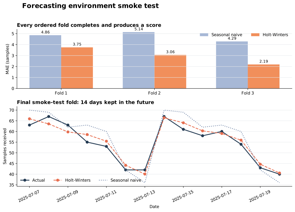
Read the bars first. Every fold produced two MAE values, so data splitting, model fitting, forecasting, and metric calculation all ran. Then inspect the lower panel. Both forecast lines follow the high weekday and low weekend rhythm. Their dates also align with the actual series instead of appearing one day early or late.

The chart is a diagnostic artifact, not decoration. An empty SVG, a missing file, or dates drawn in the wrong order means the environment has not passed.

Troubleshoot Failures One Layer at a Time

isolated environment: False. The script is using the base interpreter. Activate .venv, or call its interpreter directly with .venv/bin/python forecast_smoke_test.py on macOS or Linux and .venv\Scripts\python.exe forecast_smoke_test.py on Windows.

ModuleNotFoundError. First print sys.executable. Then run python -m pip show package-name with the same python command used for the script. Installing through a different pip is a common cause.

The frequency is None. Sort the index, look for duplicate dates, and compare it with a complete pd.date_range. Do not call .asfreq("D") and fill the new gaps until you understand why dates are missing.

A fold assertion fails. Keep the rows sorted and do not shuffle before TimeSeriesSplit. Also check that feature engineering uses only values available before each test target.

Statsmodels reports too little history. Seasonal initialization needs enough observations to estimate a cycle. Use more training data, reduce the seasonal period only when the real cycle is shorter, or test a non-seasonal model.

The optimizer warns or returns unstable results. Do not hide the warning. Record the fold, inspect the values, and try a simpler model. A smoke test should fail clearly when its forecasting layer is unreliable.

Matplotlib tries to open a window. Confirm that matplotlib.use("Agg") appears before import matplotlib.pyplot as plt. Also save the figure instead of calling plt.show() in a headless job.

Your scores differ slightly. Confirm Python and package versions, input file contents, row order, and forecast horizon. Small optimizer differences may occur across versions or platforms. The more important invariants are ordered folds, finite predictions, correct forecast length, and a successfully saved chart.

Recap: A Passing Check Is the Starting Line

A ready forecasting environment is more than a list of installed libraries. It is a tested path from one isolated interpreter through dates, ordered evaluation, model fitting, metrics, and a saved artifact.

This smoke test established that path with 196 daily observations and three future-only folds. The executed run finished with a mean Holt-Winters MAE of 3.00 samples, a mean seasonal-naive MAE of 4.76, and an accessible SVG chart. Those numbers belong only to the synthetic dataset; the durable result is that every layer produced a coherent output.

Keep the script beside your dependency file and run it after creating a new machine, updating packages, or changing a deployment image. Once it passes, replace the teaching data with a small sanitized sample of your own series and add checks for your real frequency, forecast horizon, missing-data policy, and baseline. If you need to inspect a weekly pattern before choosing a forecast, continue with weekly seasonality in pandas.