Five ARIMA orders can fit the same history, yet the fit alone does not tell you which one will predict next week most accurately. A random train-test split makes the problem worse because it lets later observations influence a model that is supposed to forecast earlier ones.

To tune ARIMA in Python, keep the observations in time order and score a small set of (p, d, q) orders with expanding-window forecasts on a validation period. Choose the lowest validation error, evaluate that order once on a later untouched test period, compare it with a simple baseline, then refit on all known data and use get_forecast() for future values and prediction intervals.

This tutorial applies that process to weekly repair requests. The task is always one week ahead: after this week’s count arrives, the service team predicts next week’s intake. The focus is model selection under realistic timing, not an automatic search through hundreds of settings.

Prerequisites and setup

You should be able to run a Python file or notebook cell. You do not need previous forecasting experience. Basic pandas knowledge is helpful, but each time-series term is defined before it is used.

Create a virtual environment, activate it, and install the four packages used in the lesson:

python -m venv .venv
source .venv/bin/activate
python -m pip install numpy pandas statsmodels matplotlib

On Windows PowerShell, activate the environment with .venv\Scripts\Activate.ps1. The published results were executed with Python 3.13.2, NumPy 2.5.1, pandas 3.0.3, statsmodels 0.14.6, and Matplotlib 3.11.0.

Download weekly_repair_requests.csv and save it beside your Python file. It contains 176 consecutive Monday observations. The repair service, dates, and counts are synthetic data created for this lesson; they do not describe a real organization. The dataset uses a fixed random seed and is released under CC0-1.0.

The lesson saves a chart rather than opening a desktop window. Select Matplotlib’s non-interactive Agg backend before importing pyplot:

import warnings

import matplotlib

matplotlib.use("Agg")

import matplotlib.pyplot as plt
import pandas as pd
from statsmodels.tools.sm_exceptions import ConvergenceWarning
from statsmodels.tsa.arima.model import ARIMA

The published outputs and chart were generated by running the reproducible lesson code.

How walk-forward validation works

An ARIMA model predicts one ordered numeric series from its own history. The name combines three parts:

• p, the number of autoregressive terms. These use earlier values of the modeled series—earlier changes when d=1—to predict its current value.
• d, the number of times the series is differenced. A first difference is current value - previous value and can remove a changing level.
• q, the number of moving-average error terms. These use information from earlier forecast errors; they are not rolling averages of the original values.

The notation ARIMA(2, 1, 0) therefore means two autoregressive terms, one round of differencing, and no moving-average error term. The current statsmodels ARIMA documentation uses the same (p, d, q) order.

Model tuning needs three ordered regions:

initial training        validation             final test
weeks 1 to 140     ->   weeks 141 to 164   ->  weeks 165 to 176
fit candidates          choose one order       check it once

Inside validation, the first forecast uses weeks 1 to 140 to predict week 141. The next forecast uses weeks 1 to 141 to predict week 142. The history expands by one actual observation each time.

This is walk-forward validation, also called time-series cross-validation. The official statsmodels forecasting guide describes the same sequence: fit on a training sample, forecast ahead, compare with later data, expand the sample, and repeat.

The final test stays outside that choice. If you keep changing the order after viewing test error, the test becomes another validation set and no longer provides a clean final check.

Load the weekly series and inspect its spacing

ARIMA depends on row order. First, parse the dates, sort them, set the date as the index, and give the series an explicit Monday frequency:

repairs = pd.read_csv(
    "weekly_repair_requests.csv",
    parse_dates=["week"],
)
repairs = repairs.set_index("week").sort_index()
series = repairs["repair_requests"].asfreq("W-MON")

print(series.head(8).to_string())
print("\nrows:", len(series))
print("frequency:", pd.infer_freq(series.index))
print("duplicate weeks:", series.index.duplicated().sum())
print("missing counts:", series.isna().sum())

The executed output is:

week
2022-01-03    60
2022-01-10    62
2022-01-17    59
2022-01-24    54
2022-01-31    49
2022-02-07    54
2022-02-14    62
2022-02-21    68
Freq: W-MON

rows: 176
frequency: W-MON
duplicate weeks: 0
missing counts: 0

W-MON means one observation per week, labeled on Monday. pandas infer_freq checks the most likely frequency from the datetime index. There are no duplicates or gaps, so moving one row means moving exactly one week.

Do not turn an unknown week into zero requests. Zero is an observed count; a missing row means the count is not available. In real data, investigate the source, repair the value when possible, or define a documented missing-data rule before fitting the model.

The level rises over the full period. Because every candidate will use d=1, inspect the first differences before fitting anything:

weekly_change = series.diff().dropna()

print(weekly_change.head(6).astype(int).to_string())
print("\nchange mean:", round(weekly_change.mean(), 2))
print("change standard deviation:", round(weekly_change.std(), 2))

week
2022-01-10    2
2022-01-17   -3
2022-01-24   -5
2022-01-31   -5
2022-02-07    5
2022-02-14    8
Freq: W-MON

change mean: 1.19
change standard deviation: 3.84

The changes move above and below zero while the average change is positive. That supports testing once-differenced models with a drift term. It does not prove that d=1 is correct for every time series. A stable, already level series may need d=0, while repeated differencing can remove useful structure.

Define a small set of ARIMA orders

Start with a short candidate list that a learner can inspect. All candidates use one difference, while p and q vary from zero to two:

CANDIDATE_ORDERS = [
    (0, 1, 0),
    (1, 1, 0),
    (0, 1, 1),
    (1, 1, 1),
    (2, 1, 0),
]

TRAIN_END = 140
VALIDATION_END = 164

With the drift term added below, ARIMA(0, 1, 0) is a simple starting point: it forecasts by extending an estimated average change. The other candidates ask whether one or two earlier changes, one earlier error, or both improve next-week predictions.

The helper below fits one order. With d=1, statsmodels does not add a trend by default. trend="t" adds a linear trend to the level, which acts like a constant drift after first differencing. That choice matches the positive average weekly change we inspected.

def fit_arima(history, order):
    with warnings.catch_warnings():
        warnings.simplefilter("ignore", ConvergenceWarning)
        return ARIMA(
            history,
            order=order,
            trend="t",
        ).fit()

The warning filter is narrow: it hides only optimizer convergence warnings during this small teaching search. In production, record these warnings and treat repeated non-convergence as a failed candidate. Do not hide every warning because date-index or numeric warnings can reveal real problems.

Score each order on future-like weeks

Now implement the expanding window. At every stop position, the code fits only the history before that position and makes one forecast. The actual value at that position is not included during fitting.

def walk_forward_predictions(data, start_position, order):
    predictions = []
    forecast_index = data.index[start_position:]

    for stop_position in range(start_position, len(data)):
        history = data.iloc[:stop_position]
        fitted = fit_arima(history, order)
        next_value = fitted.forecast(steps=1).iloc[0]
        predictions.append(float(next_value))

    return pd.Series(
        predictions,
        index=forecast_index,
        name="forecast",
    )

This refits the parameters after each actual arrives. That is slower than updating a fitted state without refitting, but it matches the weekly retraining policy in this lesson. For a large series or many candidates, first test correctness on a small search, then consider the append or extend approaches described in the statsmodels forecasting guide.

Use mean absolute error (MAE) to score all 24 validation weeks. MAE is the average absolute distance between actual and predicted counts. It stays in repair-request units, and lower is better.

def mae(actual, predicted):
    return float((actual - predicted).abs().mean())


development = series.iloc[:VALIDATION_END]
validation_actual = development.iloc[TRAIN_END:]
validation_scores = {}

for order in CANDIDATE_ORDERS:
    predicted = walk_forward_predictions(
        development,
        TRAIN_END,
        order,
    )
    validation_scores[f"ARIMA{order}"] = mae(
        validation_actual,
        predicted,
    )

score_table = pd.Series(validation_scores).sort_values()
print(score_table.round(2).to_string())

ARIMA(2, 1, 0)    2.27
ARIMA(0, 1, 1)    2.31
ARIMA(1, 1, 1)    2.33
ARIMA(1, 1, 0)    2.38
ARIMA(0, 1, 0)    2.71

ARIMA(2, 1, 0) has the lowest validation MAE, so it becomes the selected order. Its MAE of 2.27 requests is only slightly lower than those of the next two candidates. That small gap is a reason for caution: another validation period could change their ranking.

A model also needs to beat an obvious rule. The last-week baseline predicts that next week’s count will equal the latest observed count:

validation_naive = series.shift(1).iloc[TRAIN_END:VALIDATION_END]
naive_mae = mae(validation_actual, validation_naive)

print(f"selected ARIMA validation MAE: {score_table.iloc[0]:.2f}")
print(f"last-week validation MAE: {naive_mae:.2f}")

selected ARIMA validation MAE: 2.27
last-week validation MAE: 2.79

The selected ARIMA performs better than the baseline during validation. That result makes it reasonable to continue to the final test; it does not guarantee a similar improvement later.

Test the selected order once

The final 12 weeks begin on 24 February 2025. They were not used to select (2, 1, 0). Apply the same one-week-ahead update policy and compare both methods on identical dates:

SELECTED_ORDER = (2, 1, 0)

test = pd.DataFrame({
    "actual": series.iloc[VALIDATION_END:],
})
test["selected_arima"] = walk_forward_predictions(
    series,
    VALIDATION_END,
    SELECTED_ORDER,
)
test["last_week"] = series.shift(1).iloc[VALIDATION_END:]

print(test.head(6).round(1).to_string())

            actual  selected_arima  last_week
week                                          
2025-02-24     286           288.9      288.0
2025-03-03     288           284.9      286.0
2025-03-10     286           290.9      288.0
2025-03-17     285           284.3      286.0
2025-03-24     287           285.3      285.0
2025-03-31     287           289.6      287.0

Read the first row across. The actual count is 286. ARIMA predicts 288.9, while the last-week rule predicts 288. The baseline is closer for this one week, so the full-period metric is needed.

Calculate both final errors without changing the selected order:

arima_test_mae = mae(test["actual"], test["selected_arima"])
naive_test_mae = mae(test["actual"], test["last_week"])

print(f"ARIMA test MAE: {arima_test_mae:.2f} requests")
print(f"last-week test MAE: {naive_test_mae:.2f} requests")

ARIMA test MAE: 3.04 requests
last-week test MAE: 3.42 requests

Across the untouched weeks, the selected model misses by 3.04 requests per forecast on average. The baseline misses by 3.42. ARIMA keeps a small advantage, although both test errors are worse than their validation errors. This is a more honest result than reporting the best validation number as expected future performance.

Refit and forecast with a range

After evaluation, refit the selected order on all 176 known observations. statsmodels get_forecast() returns point forecasts and related results, including prediction intervals.

The next code creates eight weekly forecasts and a model-based 95% prediction interval:

final_model = fit_arima(series, SELECTED_ORDER)
forecast_result = final_model.get_forecast(steps=8)
interval = forecast_result.conf_int(alpha=0.05)

future = pd.DataFrame({
    "forecast": forecast_result.predicted_mean,
    "lower_95": interval.iloc[:, 0],
    "upper_95": interval.iloc[:, 1],
})

print(future.round(1).to_string())

            forecast  lower_95  upper_95
2025-05-19     266.4     260.9     271.9
2025-05-26     266.2     254.7     277.6
2025-06-02     267.1     250.3     283.9
2025-06-09     268.5     247.2     289.8
2025-06-16     269.9     245.0     294.8
2025-06-23     271.2     243.2     299.2
2025-06-30     272.5     241.7     303.2
2025-07-07     273.7     240.4     306.9

The first point forecast is 266.4 requests, with an interval from 260.9 to 271.9. By the eighth week, the point forecast is 273.7 and the interval has widened to 240.4–306.9. Uncertainty grows because errors can accumulate as the forecast moves farther from the last observed week.

This interval is conditional on the fitted ARIMA structure, estimated parameters, and statistical assumptions. It does not account for data-source failures, policy changes, or a sudden event that is absent from the historical pattern. The model also returns decimal forecasts for integer counts. Keep decimals for evaluation; round only when an operational display requires whole requests.

The executed build combines the ordered split, validation scores, final test, and future interval in one chart:

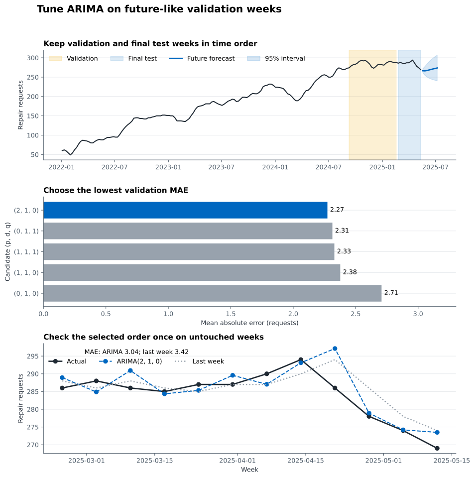
Read the middle panel first: it shows that several candidates are close, not that one order is universally correct. Then read the bottom panel to check whether the chosen order retains an advantage on untouched weeks. Finally, the top panel separates evidence from projection: shaded validation and test dates have actual values, while dates after 12 May 2025 are forecasts.

What can go wrong

Shuffling the rows. Random cross-validation trains on later weeks and tests on earlier weeks. Keep time ordered and make every forecast from information that existed before its target.

Choosing the order on the final test. Trying five orders on the test and reporting the best one uses the test for tuning. Keep a separate validation period, select once, and accept the final result even when it is disappointing.

Forgetting the baseline. An ARIMA error has little meaning without a reference. Compare it with a last-value, seasonal-naive, or another simple rule that matches the same forecast horizon. For a repeating weekly or monthly pattern, begin with seasonal naive forecasting in Python.

Changing the forecast task during evaluation. This lesson refits after every new actual and predicts one week ahead. It does not test an eight-week plan made at one fixed origin. If eight-week accuracy drives the decision, validate repeated eight-step forecasts instead.

Using d=1 by habit. Differencing a stable level can add noise. Inspect the series and its changes, use domain knowledge, and compare a small set that includes d=0 when the level is stable.

Searching too many orders on little data. A large grid can overfit the validation period. Start small, keep one final test, and prefer the simpler order when errors are practically indistinguishable.

Ignoring convergence warnings. A warning can mean the optimizer did not find a reliable solution. Record the affected orders, revise the model or use more history, and never select a candidate only because an incomplete fit produced a low score.

Treating an interval as a guarantee. The 95% range is produced by the fitted model. Check its empirical coverage across historical forecast origins before using it for capacity limits, and keep a response plan for observations outside the range.

Using non-seasonal ARIMA for clear seasonality. The candidates here do not include seasonal terms. If an hourly series repeats daily or weekly, or monthly data repeats yearly, compare a seasonal baseline and consider SARIMA rather than increasing p until the model becomes hard to maintain.

What you learned and where to go next

ARIMA tuning is a timing problem before it is a parameter problem. The durable sequence is:

1. Verify a complete, ordered time index.
2. Define the forecast horizon and update schedule.
3. Reserve validation and final test periods in the future direction.
4. Score a small candidate set with repeated future-like forecasts.
5. Select by validation error and compare with a simple baseline.
6. Check the selected order once on untouched data.
7. Refit on all known observations and report a forecast range with its limits.

For this synthetic repair series, validation selected ARIMA(2, 1, 0) at 2.27 requests MAE. On the final 12 weeks, its MAE rose to 3.04 but remained below the last-week baseline at 3.42. The exact winning order belongs to this dataset; the reusable result is the separation between selection, final checking, and future forecasting.

Next, change the operational question before changing the model. If the team plans four weeks at once, rebuild the walk-forward loop so every origin forecasts four steps and score errors by horizon. That test will answer the new decision directly instead of assuming that a strong one-week model remains strong farther ahead.