How to Tune Models for Accuracy and Speed with GridSearchCV

The highest cross-validation score can hide a costly choice. In the experiment below, an 80-tree classifier has the best average quality score, but a 20-tree alternative gives nearly the same validation quality and takes about one-third as long in the final bulk prediction benchmark.

To tune a model for accuracy and speed with GridSearchCV, score every candidate on the quality metrics that matter, define a minimum acceptable quality before seeing the test set, and use a callable refit rule to choose the fastest eligible candidate. Refit that candidate on all training rows, evaluate quality once on untouched test rows, and repeat a separate prediction-time benchmark on the hardware and batch size you plan to use.

This tutorial makes each decision visible with a random-forest classifier and fictional equipment readings. The numbers are reproducible teaching results, not evidence that any model is safe for real maintenance decisions.

Setup, files, and prerequisites

You need Python 3.11 or newer and basic knowledge of Python functions and pandas tables. A pandas DataFrame is an in-memory table with named columns. You do not need previous experience with model tuning or random forests.

Create a virtual environment, activate it, and install the packages used by the executed build:

python -m venv .venv
source .venv/bin/activate
python -m pip install numpy pandas scikit-learn matplotlib

On Windows PowerShell, activate the environment with .venv\Scripts\Activate.ps1. The published build ran with Python 3.13.2, NumPy 2.5.1, pandas 3.0.3, scikit-learn 1.9.0, and Matplotlib 3.11.0.

Download equipment_alerts.csv and save it beside your Python program or notebook. You can also inspect the complete executed grid_search_results.csv candidate table.

The input is an original synthetic dataset created deterministically for this tutorial and released under CC0-1.0. Synthetic means that code generated the rows. All 4,500 reading IDs, sensor values, and labels are fictional. The results file is derived from the executed search and is also released under CC0-1.0.

Understanding quality-constrained tuning

A hyperparameter is a setting chosen before a model learns from data. For a random forest, examples include the number of trees and the maximum depth of each tree. GridSearchCV tries every combination in a supplied grid and estimates each combination’s quality with cross-validation.

Cross-validation divides the training rows into several parts called folds. It fits a candidate on all but one fold and scores it on the remaining fold. The held-out role rotates until every fold has served as validation data. Averaging the fold scores gives a more useful comparison than one small validation split.

This lesson gives the data three separate jobs:

development rows                 test rows
      |                              |
      +-> five-fold search           +-> one final quality check
             |
             +-> apply quality and recall rules
             +-> choose the fastest eligible candidate

The final test rows stay outside tuning. Prediction speed is checked separately because cross-validation’s mean_score_time includes prediction plus scorer work inside each fold. It is useful for comparing candidates in one search, but it is not a production latency guarantee.

We will track two quality metrics:

• Balanced accuracy is the average recall across the two classes. It gives the common “no urgent inspection” class and the rare “urgent inspection” class equal influence.
• Recall for the positive class is the fraction of actual urgent cases predicted as urgent. A recall of 0.67 means the model found about 67% of positive cases.

The selection rule accepts a candidate only if its mean balanced accuracy is no more than 0.01 below the best mean balanced accuracy and its mean recall is at least 0.65. These are lesson constraints chosen before the search result was read. A real system needs limits set by domain experts, the cost of errors, and the operating environment.

Inspect the fictional alert data

Load the CSV and print a few rows before defining a model. This makes the units, target, and class balance inspectable:

import pandas as pd

alerts = pd.read_csv("equipment_alerts.csv")
print(alerts.head(6).to_string(index=False))
print("\nshape:", alerts.shape)
print(alerts["urgent_inspection"].value_counts().sort_index())

The executed output begins as follows:

reading_id  vibration_rms_mm_s  motor_temp_c  load_pct  current_variation_a  acoustic_kurtosis  days_since_service  recent_auto_stops  ambient_temp_c  urgent_inspection
  EQ-00001                1.98          49.9      22.1                 0.45                 2.26                 235                  0            34.2                  0
  EQ-00002                1.92          71.2      61.3                 2.42                 4.74                 445                  1            21.4                  1
  EQ-00003                1.90          51.1      66.3                 0.77                 3.66                 123                  0            22.3                  0
  EQ-00004                1.71          67.8      99.8                 0.72                 3.12                 375                  0            23.3                  0
  EQ-00005                2.05          73.3      81.7                 0.46                 3.65                 123                  2            29.5                  1
  EQ-00006                1.48          65.4      68.9                 1.37                 4.49                 487                  0            31.1                  1

shape: (4500, 10)
urgent_inspection
0    4058
1     442

Only 442 rows, or 9.82%, have the positive label. Plain accuracy would reward a useless model that predicts 0 for every row: it would be right 90.18% of the time while finding no urgent cases. Balanced accuracy and positive-class recall make that failure visible.

The first column is an identifier for people reading the file. It is not a sensor measurement, so exclude it from the model. Name the eight feature columns explicitly, then reserve 20% of the rows as the untouched test set:

from sklearn.model_selection import train_test_split

feature_columns = [
    "vibration_rms_mm_s",
    "motor_temp_c",
    "load_pct",
    "current_variation_a",
    "acoustic_kurtosis",
    "days_since_service",
    "recent_auto_stops",
    "ambient_temp_c",
]

X = alerts[feature_columns]
y = alerts["urgent_inspection"]

X_train, X_test, y_train, y_test = train_test_split(
    X,
    y,
    test_size=0.20,
    stratify=y,
    random_state=20260719,
)
print(X_train.shape, X_test.shape)

(3600, 8) (900, 8)

stratify=y keeps nearly the same positive-label percentage in both groups. The test set is now sealed until the model and its settings have been selected.

Search quality and timing together

A random forest combines many decision trees. n_estimators sets the number of trees. max_depth limits how many decision levels each tree can grow, while min_samples_leaf sets the minimum training rows allowed in a leaf, which is a tree’s final decision region.

The next code defines 18 combinations: three tree counts, three depth limits, and two leaf-size limits. class_weight="balanced" gives more weight to the rare class during fitting. n_jobs=1 reduces timing noise from changing levels of parallel work, and the fixed random_state makes the forest’s random choices repeatable.

from sklearn.ensemble import RandomForestClassifier
from sklearn.model_selection import GridSearchCV, StratifiedKFold

folds = StratifiedKFold(
    n_splits=5,
    shuffle=True,
    random_state=20260719,
)

forest = RandomForestClassifier(
    class_weight="balanced",
    n_jobs=1,
    random_state=20260719,
)

parameter_grid = {
    "n_estimators": [20, 80, 200],
    "max_depth": [4, 8, None],
    "min_samples_leaf": [1, 6],
}

StratifiedKFold preserves class percentages as closely as possible in each fold. That keeps the rare positive class present during every validation round. The current scikit-learn cross-validation documentation describes this behavior.

Now define the selection rule. cv_results is a dictionary containing one value per candidate. First find the best balanced accuracy and subtract 0.01. Then keep candidates that pass both the quality floor and the recall floor. Among those candidates, return the index with the lowest mean score time:

import numpy as np


def choose_fast_quality_model(cv_results):
    balanced_accuracy = np.asarray(
        cv_results["mean_test_balanced_accuracy"],
        dtype=float,
    )
    recall = np.asarray(cv_results["mean_test_recall"], dtype=float)
    score_time = np.asarray(cv_results["mean_score_time"], dtype=float)

    quality_floor = balanced_accuracy.max() - 0.01
    eligible = np.flatnonzero(
        (balanced_accuracy >= quality_floor) & (recall >= 0.65)
    )

    if len(eligible) == 0:
        return int(np.nanargmax(balanced_accuracy))
    return int(eligible[np.argmin(score_time[eligible])])

The fallback matters. If no candidate passes both requirements, the code returns the best-quality candidate instead of failing with an unclear indexing error. In a safety-critical workflow, stopping the process for human review may be the correct fallback.

Pass two scorer names and the callable to GridSearchCV, then fit only the development rows:

search = GridSearchCV(
    estimator=forest,
    param_grid=parameter_grid,
    scoring={
        "balanced_accuracy": "balanced_accuracy",
        "recall": "recall",
    },
    refit=choose_fast_quality_model,
    cv=folds,
    n_jobs=1,
)
search.fit(X_train, y_train)

The official GridSearchCV reference documents multi-metric scoring, timing columns, and callable refit. When refit is callable, best_params_, best_index_, and best_estimator_ are available, but best_score_ is not. The callable has defined the winner through a rule rather than one score.

Read the candidate table as a trade-off

Convert the search results to a DataFrame. The next step selects readable columns, changes seconds to milliseconds, and marks the chosen row:

results = pd.DataFrame(search.cv_results_)
results["cv_score_time_ms"] = results["mean_score_time"] * 1000
results["selected"] = False
results.loc[search.best_index_, "selected"] = True

shown = results.assign(
    trees=results["param_n_estimators"].astype(int),
    depth=results["param_max_depth"].fillna("unlimited"),
    leaf=results["param_min_samples_leaf"].astype(int),
).sort_values("mean_test_balanced_accuracy", ascending=False)

print(
    shown[[
        "trees",
        "depth",
        "leaf",
        "mean_test_balanced_accuracy",
        "mean_test_recall",
        "cv_score_time_ms",
        "selected",
    ]].head(8).round(4).to_string(index=False)
)

The first eight of 18 executed candidates are:

 trees     depth  leaf  mean_test_balanced_accuracy  mean_test_recall  cv_score_time_ms  selected
    80         4     1                       0.7498            0.6693            7.4086     False
   200         4     6                       0.7488            0.6636           13.9846     False
    80         4     6                       0.7477            0.6665            7.9110     False
   200         4     1                       0.7460            0.6580           14.1993     False
   200 unlimited     6                       0.7457            0.5931           20.6556     False
   200         8     6                       0.7454            0.6072           19.7263     False
    20         8     6                       0.7432            0.6157            4.3106     False
    20         4     6                       0.7407            0.6750            3.8363      True

The best mean balanced accuracy is 0.7498, so the quality floor is 0.7398. The selected 20-tree model scores 0.7407, which passes that floor, and its recall of 0.6750 passes the 0.65 recall requirement. Its mean score time is lower than the other eligible candidates.

Do not read 0.01 as “one percent slower” or “one percent worse.” Balanced accuracy is a unitless score, and the rule allows a difference of 0.01 score points. Also, the selected model’s recall is slightly higher than the best balanced-accuracy model’s recall. One metric can improve while another declines.

The generated chart shows all quality results on the left and the separate final speed measurement on the right:

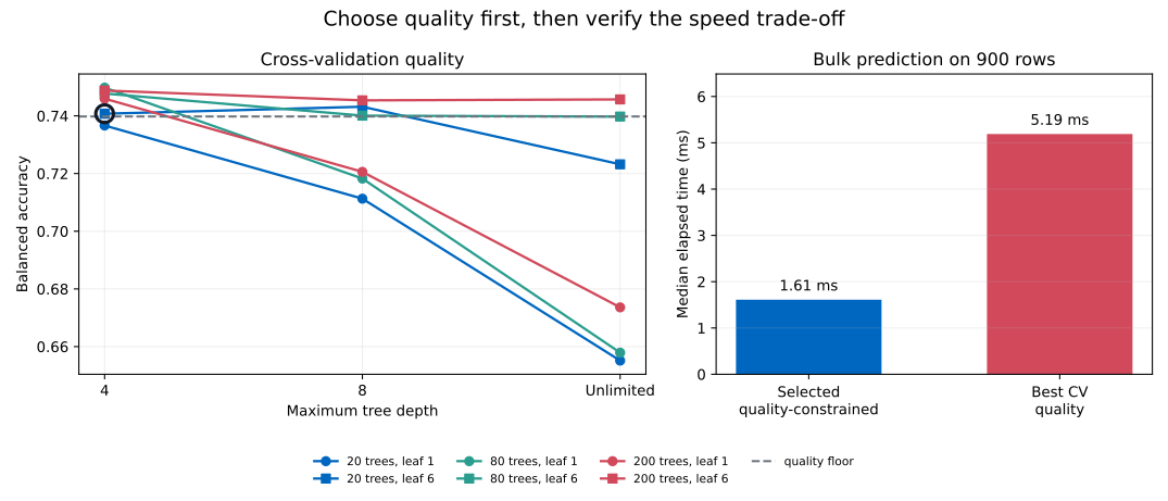
The left panel is the selection evidence. The right panel is a machine-specific check, not a promise about another computer. Official scikit-learn computational performance guidance notes that latency depends on model complexity, feature count, data representation, and whether predictions arrive singly or in batches.

Evaluate quality once, then benchmark speed

GridSearchCV has already refit the chosen configuration on all 3,600 development rows. Generate predictions for the 900 untouched test rows, then calculate the same quality metrics:

from sklearn.metrics import (
    balanced_accuracy_score,
    confusion_matrix,
    recall_score,
)

test_prediction = search.predict(X_test)

print(
    "test balanced accuracy:",
    round(balanced_accuracy_score(y_test, test_prediction), 4),
)
print("test recall:", round(recall_score(y_test, test_prediction), 4))
print("confusion matrix:")
print(confusion_matrix(y_test, test_prediction))

The executed test result is:

test balanced accuracy: 0.7859
test recall: 0.7614
confusion matrix:
[[658 154]
 [ 21  67]]

Read the confusion matrix by rows. Of 812 actual negative rows, 658 were predicted negative and 154 were false alerts. Of 88 actual positive rows, 67 were found and 21 were missed. The recall calculation is 67 / 88 = 0.7614.

The test balanced accuracy is higher than the cross-validation average. This can happen through sampling variation. It does not justify moving the quality floor or searching again. Changing the rule after seeing test results would let the test set influence tuning.

For a speed check, warm up the selected model with one prediction call. Then time the same 900-row batch 80 times and report the median, which is less affected by one unusually slow run:

from time import perf_counter


def benchmark_bulk_prediction(model, test_features):
    model.predict(test_features)  # warm-up call
    elapsed_ms = []

    for _ in range(80):
        started = perf_counter()
        model.predict(test_features)
        elapsed_ms.append((perf_counter() - started) * 1000)

    return float(np.median(elapsed_ms))


selected_ms = benchmark_bulk_prediction(search.best_estimator_, X_test)
print(f"selected model: {selected_ms:.3f} ms per 900-row batch")

The executed selected-model median was 1.610 milliseconds. The reproducible build also fitted the highest-cross-validation-quality configuration, 80 trees with depth 4 and leaf size 1, on the same training rows. Its median was 5.189 milliseconds for the same batch. On this machine and run, the higher-quality model took 3.22 times as long to predict the batch.

Repeat this benchmark in the environment that will serve predictions. Match its row batch size, input format, CPU limits, thread settings, and feature-preparation steps. If requests arrive one row at a time, a 900-row bulk benchmark answers the wrong operational question.

What can go wrong

Choosing the fastest candidate before setting a quality floor. A very small model may be quick because it learned too little. Write the quality and recall requirements first, filter with them, and compare time only inside the eligible group.

Setting requirements after reading the table. A floor chosen to make a preferred candidate win is not an independent decision rule. Record the metric, allowed gap, recall limit, and fallback before fitting the search.

Using plain accuracy with an imbalanced target. Here, 90.18% of rows are negative. A constant-negative classifier would have high accuracy and zero positive recall. Choose a metric that represents both classes and inspect the confusion matrix.

Treating mean_score_time as pure model latency. It includes prediction and scoring work on one validation fold. It is a useful same-search comparison. Benchmark the refitted candidates separately for deployment decisions.

Benchmarking each candidate once. Background tasks, cold caches, and process startup can distort one measurement. Warm up the model, repeat identical work, and summarize the distribution. For latency-sensitive services, also inspect a high percentile rather than only the median.

Using all CPU cores during a small timing comparison. Parallel work can make the order unstable when system load changes. This lesson uses one job for repeatability. Production tuning should test the thread and process limits that the deployed service will actually have.

Tuning on the test set. Do not compare all 18 test scores or speed results and then choose again. The test set grades the completed selection. If the requirements change, create a new evaluation plan and obtain genuinely untouched data.

Ignoring preprocessing cost. Database reads, parsing, missing-value handling, and feature creation may take longer than predict(). Time the complete request path before making an operational claim. If your data needs scaling, keep preprocessing inside a leakage-safe pipeline; How to Compare Data Scalers with Cross-Validation in Python shows that structure.

Applying random folds to grouped or ordered rows. The fictional readings are independent. Real sensor data may contain many rows from one machine or a time sequence. Use group-aware or time-aware validation so closely related rows do not cross the training-validation boundary.

Recap: turn tuning into a written decision

Model tuning is clearer when it produces a decision, not only a leaderboard. In this lesson, five-fold cross-validation evaluated 18 random forests on balanced accuracy and recall. A rule kept candidates within 0.01 of the best balanced accuracy, required at least 0.65 recall, and used mean validation score time only after those quality checks.

That rule selected 20 trees with depth 4 and a minimum leaf size of 6. Its test balanced accuracy was 0.7859, its test recall was 0.7614, and it found 67 of 88 positive test cases. On the build machine, its median 900-row prediction time was about one-third of the highest-validation-quality model’s time.

The reusable method is short: reserve test data, state quality constraints, collect every relevant metric, select within the eligible set, and verify both quality and speed under realistic conditions. The numerical winner will change with the data and hardware. The written decision rule is the durable part.