Find Weekly Seasonality in Python with pandas Rolling Windows

A support team receives more requests on some days than others. A high count may mean that the service has a problem. It may also be a normal Monday. If you compare every day with one overall average, you cannot tell the difference.

This tutorial shows how to find a weekly pattern in daily data with pandas. We will separate each observation into a slow-moving baseline, a normal weekday adjustment, and a leftover value. That leftover value helps us distinguish a recurring calendar effect from a day that deserves investigation.

The goal is analysis, not forecasting. We will build a transparent baseline that a beginner can inspect. For a broader first-pass routine before working with dates, see the exploratory data analysis with pandas tutorial.

What You Need Before You Begin

You should be comfortable running a Python script or a notebook cell. You do not need previous time-series knowledge. A time series is simply a set of observations arranged by time, such as one request count per day.

Create a virtual environment if you want an isolated project, then install the two packages used in the analysis:

python -m venv .venv
source .venv/bin/activate
python -m pip install pandas matplotlib

On Windows PowerShell, activate the environment with .venv\Scripts\Activate.ps1 instead. The published results use Python 3.13.2, pandas 3.0.3, and Matplotlib 3.11.0. NumPy 2.5.1 was used only to generate the downloadable synthetic dataset.

Download support_requests.csv into your working folder. It contains 168 consecutive daily observations, or exactly 24 weeks, from 6 January to 22 June 2025. The counts, dates of unusual events, and organization are fictional. The dataset was generated with a fixed random seed and is released under CC0-1.0, so you may reuse it without restriction.

The dates are historical only to make the example concrete. They do not describe a real support service.

The Mental Model: Baseline, Calendar Pattern, Leftover

We will treat a daily count as the sum of three parts:

observed requests = moving baseline + weekday effect + residual

The moving baseline is the slow change underneath the daily movement. The support service may gain users over several months, so its normal request count can rise.

The weekday effect is the recurring weekly pattern. For example, Mondays may usually sit above the baseline while Saturdays sit below it. This part repeats every seven observations because the data has one row per day.

The residual is what remains after subtracting the first two parts. Residual does not mean error in the code. It means variation that our simple baseline and weekday pattern do not explain.

This is an additive model because the parts are added in the same request-count units. A Monday adjustment of +17 means about 17 requests above the moving baseline, whether the baseline is 75 or 95. If the weekly swing grew in proportion to the level, a log transform or a different model could be more suitable.

This workflow depends on two choices that come from the data, not from pandas. We choose seven observations because daily data has a seven-day week. We use a centered window because the purpose is to explain existing history, not to predict tomorrow.

Load and Check the Daily Series

First, load the CSV, parse the date strings as real datetime values, and make the date the index. A DatetimeIndex is pandas’ date-aware row label. It lets us ask calendar questions later.

import pandas as pd
import matplotlib.pyplot as plt

support = pd.read_csv("support_requests.csv", parse_dates=["date"])
support = support.set_index("date")

print(support.head(8).to_string())
print("\nshape:", support.shape)
print("ordered:", support.index.is_monotonic_increasing)

            requests
date                
2025-01-06        87
2025-01-07        86
2025-01-08        76
2025-01-09        74
2025-01-10        71
2025-01-11        50
2025-01-12        60
2025-01-13        88

shape: (168, 1)
ordered: True

There is one numeric column and 168 ordered rows. Even this small preview hints at a weekly shape: the first Monday has 87 requests, while the first Saturday has 50. One week is not enough evidence, so we will estimate the pattern across all 24 weeks.

Check that the dates are unique and one day apart before calculating a seven-row window:

print("duplicate dates:", support.index.duplicated().sum())
print("daily frequency:", pd.infer_freq(support.index))
print("missing counts:", support["requests"].isna().sum())

duplicate dates: 0
daily frequency: D
missing counts: 0

D means daily frequency. This check matters because a seven-row window represents a week only when every row represents one consecutive day. The pandas time-series guide also recommends a sorted date index because some date operations can behave unexpectedly on unsorted data.

Estimate the Moving Baseline

A rolling mean averages a window that moves through the rows. Here, each window contains seven days. Centering places the result on the middle date, so the trend for Thursday uses the surrounding Monday-to-Sunday week.

support["trend"] = support["requests"].rolling(
    window=7,
    center=True,
    min_periods=7,
).mean()

print(support[["requests", "trend"]].head(9).round(2).to_string())
print("\nmissing trend values:", support["trend"].isna().sum())

            requests  trend
date                       
2025-01-06        87    NaN
2025-01-07        86    NaN
2025-01-08        76    NaN
2025-01-09        74  72.00
2025-01-10        71  72.14
2025-01-11        50  71.29
2025-01-12        60  72.14
2025-01-13        88  71.43
2025-01-14        80  70.71

missing trend values: 6

The first three and last three trend values are missing. A full centered seven-day window needs three observations before and three after the current day. pandas returns NaN, meaning a missing numeric value, when that full window is unavailable. The current rolling documentation defines center=True as labeling each result at the window center and min_periods as the minimum observations required.

The trend around the first complete week is about 72 requests. Averaging a complete seven-day cycle reduces the Monday-to-weekend swing while retaining the slower rise across months.

Measure the Normal Effect of Each Weekday

Next, subtract the trend from each observation. This operation is called detrending. It prevents the later, busier weeks from making every weekday look artificially high.

We then group the detrended values by weekday and take their mean. pandas numbers Monday as 0 and Sunday as 6, but day_name() gives readable labels.

support["detrended"] = support["requests"] - support["trend"]
support["weekday"] = support.index.day_name()

weekday_order = [
    "Monday", "Tuesday", "Wednesday", "Thursday",
    "Friday", "Saturday", "Sunday",
]

seasonal_profile = (
    support.groupby("weekday")["detrended"]
    .mean()
    .reindex(weekday_order)
)
seasonal_profile = seasonal_profile - seasonal_profile.mean()

print(seasonal_profile.round(2).to_string())
print("\nprofile mean:", round(seasonal_profile.mean(), 10))

weekday
Monday       17.09
Tuesday      10.43
Wednesday     5.24
Thursday      1.30
Friday       -3.68
Saturday    -17.04
Sunday      -13.34

profile mean: 0.0

Read each number as an adjustment to the moving baseline. A typical Monday is about 17.09 requests above the baseline. A typical Saturday is about 17.04 below it. The adjustments average to zero, so they move requests between weekdays without changing the overall level.

Why subtract seasonal_profile.mean()? Small noise and incomplete edge windows can leave the seven grouped means slightly off center. Recentering makes the interpretation exact: the trend holds the level, and the weekday profile only describes the repeating shape.

Rebuild Expected Demand and Find Unusual Days

Now map each weekday adjustment back to every row. Add it to the trend to calculate expected requests. Then subtract expected requests from observed requests to get the residual.

support["seasonal"] = support["weekday"].map(seasonal_profile).astype(float)
support["expected"] = support["trend"] + support["seasonal"]
support["residual"] = support["requests"] - support["expected"]

usable = support.dropna(subset=["trend", "residual"])
residual_std = usable["residual"].std()
threshold = 2.5 * residual_std
unusual = usable.loc[usable["residual"].abs() > threshold]

print("residual standard deviation:", round(residual_std, 2))
print("threshold:", round(threshold, 2))
print(unusual[["requests", "expected", "residual"]].round(1).to_string())

residual standard deviation: 5.08
threshold: 12.7
            requests  expected  residual
date                                    
2025-02-20       111      86.3      24.7
2025-04-19       109      78.0      31.0
2025-06-01       115      85.8      29.2

The standard deviation measures the typical spread of residuals around zero. We mark values farther than 2.5 standard deviations from zero as unusual. This is a practical screening rule, not a universal law and not proof of an incident.

The second row shows why the weekday adjustment helps. On 19 April, the service received 109 requests. That date was a Saturday, so its expected value was only 78.0 after accounting for the normal weekend drop. The positive residual of 31.0 is much more informative than a comparison with one global average.

The three dates were deliberately added to this synthetic dataset as fictional service incidents. In real work, the result should start an investigation. Check deployments, outages, campaigns, missing records, and changes in how requests were counted.

Plot the Three Parts Together

The following code plots the calculations from the previous sections. The top panel compares observed requests with the rolling baseline. The middle panel shows the weekday profile. The bottom panel shows the residuals and marks values beyond the threshold.

fig, axes = plt.subplots(3, 1, figsize=(10, 8))

axes[0].plot(
    support.index, support["requests"],
    color="#4C78A8", linewidth=1.2, label="Observed",
)
axes[0].plot(
    support.index, support["trend"],
    color="#E45756", linewidth=2.2, label="7-day trend",
)
axes[0].set_title("Observed requests and the slow-moving baseline", loc="left")
axes[0].set_ylabel("Requests")
axes[0].legend(frameon=False, ncol=2, loc="upper left")

bar_colors = [
    "#F58518" if value > 0 else "#54A24B"
    for value in seasonal_profile
]
axes[1].bar(weekday_order, seasonal_profile, color=bar_colors)
axes[1].axhline(0, color="#555555", linewidth=0.8)
axes[1].set_title(
    "Typical weekday adjustment after removing the trend", loc="left"
)
axes[1].set_ylabel("Requests above/below trend")
axes[1].tick_params(axis="x", rotation=25)

axes[2].plot(
    usable.index, usable["residual"], color="#7A5195", linewidth=1.1
)
axes[2].axhline(threshold, color="#777777", linestyle="--", linewidth=1)
axes[2].axhline(-threshold, color="#777777", linestyle="--", linewidth=1)
axes[2].scatter(
    unusual.index, unusual["residual"],
    color="#D62728", s=36, zorder=3, label="Unusual day",
)
axes[2].set_title(
    "Leftover variation after trend and weekday effects", loc="left"
)
axes[2].set_ylabel("Residual requests")
axes[2].set_xlabel("Date")
axes[2].legend(frameon=False, loc="upper left")

for ax in axes:
    ax.spines[["top", "right"]].set_visible(False)
    ax.grid(axis="y", color="#DDDDDD", linewidth=0.6)

fig.suptitle(
    "Separate a weekly pattern from changing support demand",
    fontsize=15, fontweight="bold", x=0.08, ha="left",
)
fig.tight_layout(rect=(0, 0, 1, 0.97))
fig.savefig(
    "weekly-seasonality-pandas-components.svg",
    format="svg",
    bbox_inches="tight",
)

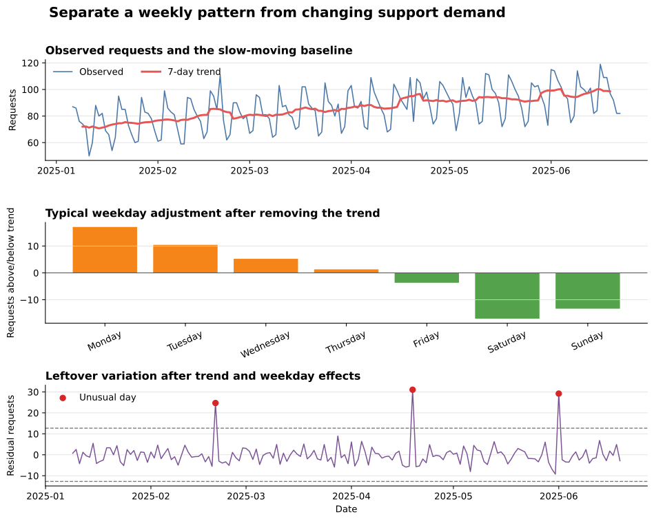
Start with the middle panel. Its strong Monday-to-weekend slope confirms that weekday is useful context. Then inspect the top panel: the baseline rises slowly, so one fixed average would become stale. Finally, read the bottom panel. Most residuals stay close to zero, while three points cross the upper dashed line.

Common Mistakes and Troubleshooting

Using seven rows when rows are not daily. If dates are missing, seven rows may span eight or more days. Reindex to a complete daily range and decide how missing values should be handled before using a row-count window. Never replace a missing count with zero unless zero truly means no requests.

Forgetting to sort the date index. A rolling window follows row order. Run support = support.sort_index() and check duplicates before calculating the trend.

Treating a centered trend as a forecast feature. The centered value uses future observations. That is appropriate for explaining completed history, but it leaks future information into a prediction task. For forecasting, use a trailing window with center=False and calculate every feature using only information available at prediction time.

Choosing the period from habit. Seven is correct here because each observation is one day and the operational cycle is weekly. Hourly data may have daily and weekly patterns. Monthly data may have a 12-month pattern. Plot the data and use domain knowledge before choosing a window.

Calling every large residual an incident. A threshold ranks observations for review; it does not explain them. Holidays, reporting changes, one-time events, and data errors can all produce large residuals.

Ignoring a changing seasonal size. This example assumes the weekday adjustment stays roughly constant in request units. If Monday’s extra demand grows as the service grows, compare ratios or log-transformed counts, or use a model designed for changing seasonal strength.

Recap and Next Step

You can make a daily series easier to interpret with three direct pandas operations:

1. Use a centered seven-day rolling mean to estimate the moving baseline in completed historical data.
2. Subtract that baseline, then average by weekday to estimate the recurring weekly effect.
3. Subtract both parts to obtain residuals, then review values that are large compared with normal residual variation.

The durable idea is comparison with the right expectation. A busy Monday can be normal, while the same count on Saturday can be unusual. Trend supplies the current level, the calendar pattern supplies the local context, and the residual shows what those two parts did not explain.

For a real service, the next step is to add known context such as holidays, product releases, and outages. Keep those labels separate from the residual calculation at first. You can then test whether the unexplained dates match events the team already knows about and decide whether the baseline is useful for monitoring.