What Is Scikit-learn, and How Does It Fit Into AI?

Type “what is scikit-learn” into a search bar and you’ll get some version of the same two-line answer: it’s a Python library for machine learning. True, but it doesn’t tell you anything you can act on. It doesn’t say what jobs the library actually does, why it isn’t the neural-network kind of thing people usually mean when they say “AI” these days, or when you’d reach for it instead of TensorFlow. That’s the gap this post fills.

Scikit-learn is a free, open-source Python library that implements the classical side of machine learning — algorithms that learn statistical and geometric patterns from structured, tabular data, rather than the layered neural networks behind large language models and image generators. In a real AI project it’s usually the tool doing classification, regression, clustering, and dimensionality reduction, plus the data-preparation work around all four, while a separate deep-learning framework handles anything built from neural network layers. Both live under the same “AI” umbrella; they solve different shapes of problem, with very different amounts of data and compute.

If you already know scikit-learn’s shared fit/predict/transform rhythm cold, our deep dive on that interface covers it in more depth than this post will. Here the question is bigger picture: what can this library actually do, and where does it sit relative to everything else people call “AI”?

The Shape of the AI Toolbox

“AI” is a big, loose umbrella. Machine learning is the part of it where a system improves at a task by learning from data instead of being programmed rule by rule. Deep learning is one way to do machine learning — stacking layers of a neural network and training all of them together, which is what powers modern language and image models. Classical machine learning is the other way: statistical and geometric algorithms — nearest neighbors, linear models, decision trees, k-means — that learn directly from a table of numbers, usually far faster and on far less data than a neural network needs.

Scikit-learn is the standard Python library for the classical side. It doesn’t build or train neural networks — that’s TensorFlow and Keras territory. What it does cover is nearly everything else a tabular-data project needs, organized into a small number of task families that all share the same fit-then-do-something call shape:

• Classification — assign each row a category
• Regression — predict a number
• Clustering — group similar rows with no labels at all
• Dimensionality reduction — compress many columns into fewer, information-dense ones
• Model selection & preprocessing — the utilities (train_test_split, StandardScaler, Pipeline, cross_val_score) that make any of the above trustworthy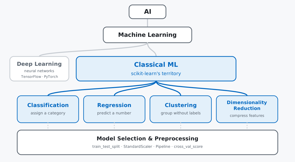

Scikit-learn’s own documentation actually draws this as a literal flowchart — the “choosing the right estimator” map starts with “do you have labels?” and routes you toward classification, regression, or clustering from there. The rest of this post walks that same map on one real dataset, in order: classification, then clustering, then dimensionality reduction, then the glue that ties them together.

The Data: 569 Tumors, 30 Measurements

Rather than inventing numbers, this post uses a real diagnostic dataset that ships with scikit-learn itself, so nothing here needs downloading or an account. Picture a pathology lab that has photographed a fine-needle aspirate of a breast mass and measured properties of the cell nuclei visible in the image — radius, texture, smoothness, and so on — computing the mean, standard error, and worst (largest) value for each of ten base measurements, for 30 numeric features per sample. The question a classifier answers: do this sample’s measurements look malignant or benign?

Data: the Breast Cancer Wisconsin (Diagnostic) dataset bundled with scikit-learn (originally donated to the UCI Machine Learning Repository; redistributed here under scikit-learn’s own BSD license), loaded via load_breast_cancer(). (The outputs in this post come from pandas 3.0.3, numpy 2.5.1, and scikit-learn 1.9.0.)

import pandas as pd
from sklearn.datasets import load_breast_cancer

data = load_breast_cancer(as_frame=True)
df = data.frame
df[["mean radius", "mean texture", "mean area", "worst radius", "target"]].head()

   mean radius  mean texture  mean area  worst radius  target
0        17.99         10.38     1001.0         25.38       0
1        20.57         17.77     1326.0         24.99       0
2        19.69         21.25     1203.0         23.57       0
3        11.42         20.38      386.1         14.91       0
4        20.29         14.34     1297.0         22.54       0

df.shape

(569, 31)

569 samples, 30 features plus the target column. target is 0 or 1, and data.target_names says which is which:

data.target_names

['malignant' 'benign']

df["target"].value_counts().sort_index()

target
0    212
1    357
Name: count, dtype: int64

212 malignant samples, 357 benign — not a rare-event problem, but not perfectly even either. One more thing worth checking before any modeling: do the 30 features share a common scale?

df[["mean area", "mean smoothness"]].describe().round(3)

       mean area  mean smoothness
count    569.000          569.000
mean     654.889            0.096
std      351.914            0.014
min      143.500            0.053
25%      420.300            0.086
50%      551.100            0.096
75%      782.700            0.105
max     2501.000            0.163

They don’t. mean area ranges into the thousands with a standard deviation of 351.9; mean smoothness lives in a tight band under 0.2 with a standard deviation of 0.014 — roughly 25,000 times smaller. Keep that gap in mind; it comes back later.

Teaching a Model to Tell Malignant from Benign

Classification is the task family most people picture first: given a row of features, output one of a fixed set of categories. Set aside a test set the model never trains on, scale the features, and fit a classifier:

from sklearn.model_selection import train_test_split
from sklearn.preprocessing import StandardScaler
from sklearn.linear_model import LogisticRegression
from sklearn.metrics import accuracy_score

X = df.drop(columns=["target"])
y = df["target"]

X_train, X_test, y_train, y_test = train_test_split(
    X, y, test_size=0.2, random_state=42, stratify=y
)
print(X_train.shape, X_test.shape)

(455, 30) (114, 30)

stratify=y keeps the same 212:357 ratio in both slices, so an unlucky shuffle can’t leave the test set thin on one class. Scaling happens next — fit only on the training rows, then applied to both:

scaler = StandardScaler()
X_train_scaled = scaler.fit_transform(X_train)
X_test_scaled = scaler.transform(X_test)

clf = LogisticRegression(max_iter=10000)
clf.fit(X_train_scaled, y_train)
y_pred = clf.predict(X_test_scaled)

acc = accuracy_score(y_test, y_pred)
print(f"accuracy: {acc:.3f}")

accuracy: 0.982

98.2% on 114 held-out samples. Accuracy alone hides which class gets missed, so break it down per class:

from sklearn.metrics import classification_report

print(classification_report(y_test, y_pred, target_names=data.target_names))

              precision    recall  f1-score   support

   malignant       0.98      0.98      0.98        42
      benign       0.99      0.99      0.99        72

    accuracy                           0.98       114
   macro avg       0.98      0.98      0.98       114
weighted avg       0.98      0.98      0.98       114

Both classes score close to 1.00 on precision and recall, and the support column confirms the split held its 42:72 proportion (matching the roughly 2:3.5 ratio from the full dataset). This is what “classification” means end to end: configure an estimator, fit it on labeled training rows, predict labels for rows it never saw, then grade those predictions against the truth.

Finding Structure Without Being Told the Answer

Clustering is a different job entirely: no y, no labels, no “correct” answer to train toward. You hand the algorithm a table of features and ask it to group similar rows together based on the features alone. Unlike a classifier, a clustering model doesn’t need a held-out test set to grade itself against — there’s no label being predicted that could leak from training — so it’s reasonable to fit it on every row:

from sklearn.cluster import KMeans
from sklearn.metrics import adjusted_rand_score
import numpy as np

X_all_scaled = scaler.fit_transform(X)

kmeans = KMeans(n_clusters=2, random_state=42, n_init=10)
cluster_labels = kmeans.fit_predict(X_all_scaled)

print("cluster sizes:", np.bincount(cluster_labels))
print("true label sizes:", np.bincount(y))

cluster sizes: [375 194]
true label sizes: [212 357]

The cluster sizes (375 and 194) don’t match the true label sizes (212 and 357) — no surprise, since KMeans never saw target at all. What it’s worth checking is whether the two clusters line up with the real diagnosis anyway, purely because malignant and benign tumors tend to look different in feature space:

ari = adjusted_rand_score(y, cluster_labels)
print(f"adjusted rand index vs true diagnosis: {ari:.3f}")

adjusted rand index vs true diagnosis: 0.654

adjusted_rand_score scores 1.0 for a perfect match and roughly 0.0 for a random grouping; 0.654 says these unsupervised clusters correlate strongly with the real diagnosis, without ever being told what to look for. A crosstab shows exactly where they agree and disagree:

print(pd.crosstab(y, cluster_labels, rownames=["true_target"], colnames=["cluster"]))

cluster        0    1
true_target          
0             36  176
1            339   18

Cluster 1 catches 176 of the 212 malignant samples; cluster 0 catches 339 of the 357 benign ones. But 36 malignant samples land in the “benign-leaning” cluster and 18 benign samples land in the “malignant-leaning” one. Clustering found real structure in the data — it did not accidentally reinvent a diagnosis.

Shrinking 30 Features Down to Two

The third task family, dimensionality reduction, solves a different problem again: 30 correlated columns are hard to plot, slow to search over, and often redundant (mean radius and mean area are practically the same information twice). Principal Component Analysis (PCA) builds a small number of new columns — components — that capture as much of the original variance as possible:

from sklearn.decomposition import PCA

pca = PCA(n_components=2, random_state=42)
X_pca = pca.fit_transform(X_all_scaled)

print("explained variance ratio:", np.round(pca.explained_variance_ratio_, 3))
print("total variance captured:", round(pca.explained_variance_ratio_.sum(), 3))

explained variance ratio: [0.443 0.19 ]
total variance captured: 0.632

Two components, built from all 30 scaled features, retain 63.2% of the dataset’s total variance — enough to plot every sample on an ordinary 2D scatterplot and still see real separation between groups, even though it’s nowhere near enough to replace the full feature set for a serious model:

pd.DataFrame(X_pca[:5], columns=["pc1", "pc2"]).round(2)

    pc1    pc2
0  9.19   1.95
1  2.39  -3.77
2  5.73  -1.08
3  7.12  10.28
4  3.94  -1.95

Each row here is one 30-number tumor measurement, rewritten as just two numbers. .fit_transform() — the same verb StandardScaler used earlier — is doing the same job here: learn something from X, then reshape X according to what it learned.

The Glue That Holds a Real Workflow Together

None of the three sections above worked in isolation — each one leaned on StandardScaler, train_test_split, or both. In a real project you don’t run these by hand and hope you did it consistently every time; you chain them into one object and validate the whole thing at once:

from sklearn.pipeline import Pipeline
from sklearn.model_selection import cross_val_score

pipe = Pipeline([
    ("scaler", StandardScaler()),
    ("clf", LogisticRegression(max_iter=10000)),
])
scores = cross_val_score(pipe, X, y, cv=5)

print("fold scores:", np.round(scores, 3))
print(f"mean cv accuracy: {scores.mean():.3f} (+/- {scores.std():.3f})")

fold scores: [0.982 0.982 0.974 0.974 0.991]
mean cv accuracy: 0.981 (+/- 0.007)

cross_val_score repeats the split-scale-fit-score cycle five times on five different train/test partitions and reports each fold’s accuracy. 0.981 average is close to the single 0.982 split from earlier, but it’s a steadier number, and it comes with zero risk of scaling leakage: Pipeline re-fits the scaler fresh inside each fold, on that fold’s training rows only. This fit/predict/transform shape — one object, one method call, whatever the underlying job — is the same idea our scikit-learn overview post covers estimator by estimator; here it’s just the connective tissue between three otherwise-separate task families.

Where This Shows Up in a Bigger AI System

None of this requires a neural network anywhere in the picture, and that’s the point: a huge share of real-world “AI” work is still classical machine learning, quietly, because the data is tabular and the classical tools are faster to train, easier to explain to a stakeholder, and cheap enough to run on a laptop instead of a GPU cluster. Scikit-learn also shows up inside projects that do use deep learning, doing jobs that have nothing to do with neural networks themselves: train_test_split builds the held-out evaluation set for almost any model, classical classifiers give you a fast baseline to beat before justifying a much more expensive neural network, and metrics like classification_report or adjusted_rand_score grade a model’s output regardless of what produced it. If you’ve ever seen a data science project described as “80% data preparation,” a large share of that 80% runs through exactly the utilities this post just used.

Where the Convenient Story Breaks

Unscaled features quietly distort anything based on distance or variance. PCA and KMeans both rely on distances and spread between points — and both get misled by a column like mean area sitting on a completely different scale than mean smoothness:

pca_unscaled = PCA(n_components=2, random_state=42)
X_pca_unscaled = pca_unscaled.fit_transform(X)
print("explained variance ratio (unscaled):", np.round(pca_unscaled.explained_variance_ratio_, 3))

explained variance ratio (unscaled): [0.982 0.016]

kmeans_unscaled = KMeans(n_clusters=2, random_state=42, n_init=10)
cluster_labels_unscaled = kmeans_unscaled.fit_predict(X)
ari_unscaled = adjusted_rand_score(y, cluster_labels_unscaled)
print(f"adjusted rand index (unscaled features): {ari_unscaled:.3f}")
print(f"adjusted rand index (scaled features):   {ari:.3f}")

adjusted rand index (unscaled features): 0.491
adjusted rand index (scaled features):   0.654

Unscaled, PCA’s first component alone claims 98.2% of the variance — not because one direction in the data is genuinely that dominant, but because mean area’s huge raw values swamp everything else in the variance calculation. Clustering suffers the same way: the adjusted Rand index drops from 0.654 to 0.491 once features go back to their raw, mismatched scales. Any algorithm that measures distance or spread needs scaled input; only algorithms based purely on splits (decision trees, most tree ensembles) are naturally immune.

Clustering isn’t classification, even when the numbers look close. A 0.654 adjusted Rand index is a real, useful signal — but it’s not “97% accuracy” wearing a disguise. The crosstab above showed 36 malignant and 18 benign samples landing in the “wrong” cluster; a clustering algorithm has no mechanism to know it got those wrong, because it was never shown a right answer in the first place. Treat clustering as a way to discover structure, not a substitute for a trained classifier.

Scikit-learn doesn’t do deep learning, and isn’t trying to. It ships MLPClassifier, a basic multi-layer perceptron, but nobody trains a modern computer-vision or language model on it — there’s no GPU acceleration, no automatic differentiation, and no support for the transformer or convolutional architectures those models are built from. Once your data is unstructured (raw images, audio, long text) or your dataset is enormous, that’s the boundary where TensorFlow, Keras, and neural networks take over from everything in this post.

The Short Version

Classical machine learning (scikit-learn) and deep learning (TensorFlow, PyTorch) are both “AI,” solving different shapes of problem: tabular data and modest compute on one side, unstructured data and heavy compute on the other. Inside scikit-learn’s half, four task families cover almost everything — classification, regression, clustering, and dimensionality reduction — held together by preprocessing and model-selection utilities that make the results trustworthy rather than accidental. Every number above came from one dataset, verified end to end: 98.2% single-split accuracy, 98.1% average cross-validated accuracy, a 0.654 adjusted Rand index from clustering with zero labels, and 63.2% of 30 features’ variance surviving compression to two.

If you want the guided, from-scratch version of the classification example above — same dataset, a k-nearest neighbors model instead of logistic regression, and a full confusion-matrix and ROC evaluation — the Guided Project: Predicting Breast Cancer Diagnosis lesson picks it up from exactly here. For the clustering side, K-Means with Scikit-Learn and Interpreting Results turns unlabeled customer data into a real segmentation story the same way we just clustered tumor measurements. Both lessons live inside our free Machine Learning course, which covers the deep-learning half of this landscape too.