An attention calculation may look reasonable with four query features, then become almost a winner-takes-all choice with 1,024 features. The code did not change. Only the vector width changed.

Scale dot-product attention by dividing every query-key score by sqrt(d_k) before softmax, where d_k is the shared width of each query and key. If their components have roughly stable variance, an unscaled dot product’s standard deviation grows like sqrt(d_k); the division removes that width-driven growth and keeps softmax from becoming sharp only because the vectors are wider.

This tutorial tests that answer with NumPy instead of asking you to accept the formula. We will follow one four-dimensional query across four scores, predict what should happen as width grows, and run 20,000 synthetic trials. If queries, keys, and values are new terms, first read scaled dot-product attention in NumPy. This lesson isolates the scaling step.

Setup and prerequisites

You need Python 3.11 or newer. You should be comfortable with Python functions and one-dimensional NumPy arrays. Basic knowledge of averages is enough; the variance terms are explained before they are used.

Create a virtual environment and install the packages used by the executed lesson:

python -m venv .venv
source .venv/bin/activate
python -m pip install numpy pandas matplotlib

On Windows PowerShell, activate the environment with .venv\Scripts\Activate.ps1. The executed results used Python 3.13.2, NumPy 2.5.1, pandas 3.0.3, and Matplotlib 3.11.0.

The experiment creates its own numbers with a fixed random seed. It does not use language, customer, or sensor data. Its queries and keys are synthetic samples from a standard normal distribution, which has mean 0 and standard deviation 1. The generated attention scaling results CSV is released under CC0-1.0.

Start with these imports. Matplotlib’s Agg backend saves a real SVG without trying to open a desktop window, so select it before importing pyplot:

import matplotlib

matplotlib.use("Agg")

import matplotlib.pyplot as plt
import numpy as np
import pandas as pd

The published chart and CSV were produced by the same executed Python build as the printed results below.

How score scaling works as width grows

In dot-product attention, a query is compared with a key by multiplying values in matching positions and adding the products. If both vectors contain four numbers, the score has four terms:

score = q[0]×k[0] + q[1]×k[1] + q[2]×k[2] + q[3]×k[3]

At width 1,024, the same operation adds 1,024 terms. Even if positive and negative products often cancel, the score distribution spreads farther from zero as more independent terms are added.

The phrase standard deviation describes that spread around the average. Under the simple assumptions used in this experiment, each query and key component is independent, has mean 0, and has variance 1. Variance is the square of standard deviation. Each query-key product then has variance 1, so a sum of d_k independent products has variance d_k:

variance(raw score) = d_k
standard deviation(raw score) = sqrt(d_k)

Now divide the score by its predicted standard deviation:

standard deviation(raw score / sqrt(d_k)) = 1

This is the key idea. Scaling does not make every score small or every attention row uniform. It removes the automatic increase caused by vector width under these assumptions. The learned query-key relationships can still make one score larger than another.

The original Transformer paper gives the same variance argument and notes that large scores can push softmax into regions where its gradients are very small. Current PyTorch scaled-dot-product attention documentation uses 1 / sqrt(E) as its default scale, where E is the query and key width.

Follow one four-dimensional comparison

Before running thousands of trials, inspect one small row. The next function implements stable softmax. Softmax changes a row of scores into positive weights that sum to 1. Subtracting the largest score first keeps the exponentials within a safer numeric range without changing the weights.

def stable_softmax(scores):
    shifted = scores - scores.max(axis=-1, keepdims=True)
    exponentials = np.exp(shifted)
    return exponentials / exponentials.sum(axis=-1, keepdims=True)

Use one query and four keys. Each vector has width 4, so sqrt(d_k) equals 2. The matrix multiplication calculates all four query-key scores in one operation:

query = np.array([1.0, -1.0, 0.5, 0.5])
keys = np.array([
    [1.0, 0.0, 1.0, 0.0],
    [0.0, 1.0, 0.0, 1.0],
    [1.0, -1.0, 0.5, 0.5],
    [0.5, -0.5, -1.0, 1.0],
])

raw_scores = query @ keys.T
scaled_scores = raw_scores / np.sqrt(query.size)

print("raw scores:", raw_scores)
print("scaled scores:", scaled_scores)
print("raw weights:", np.round(stable_softmax(raw_scores), 3))
print("scaled weights:", np.round(stable_softmax(scaled_scores), 3))

The executed output is:

raw scores: [ 1.5 -0.5  2.5  1. ]
scaled scores: [ 0.75 -0.25  1.25  0.5 ]
raw weights: [0.224 0.03  0.609 0.136]
scaled weights: [0.263 0.097 0.434 0.205]

The third key still receives the largest weight after scaling. Its lead is smaller: the weight changes from 0.609 to 0.434. Scaling preserves score order because every score is divided by the same positive number. It changes the gaps that softmax sees, not which raw score ranks first.

This four-number example shows the immediate effect, but it cannot show whether the rule stays useful at other widths. For that, we need repeated trials.

Measure five query and key widths

The experiment uses widths 4, 16, 64, 256, and 1,024. For each width, it generates 4,000 queries. Every query is compared with 12 independently generated keys. That produces 48,000 scores per width and 240,000 scores in total.

NumPy recommends a Generator created by default_rng for new random code. A fixed seed makes this run repeatable with the tested environment:

WIDTHS = [4, 16, 64, 256, 1024]
TRIALS = 4_000
KEY_COUNT = 12
BATCH_SIZE = 200

rng = np.random.default_rng(20_260_718)

Generate the widest arrays in batches so the lesson does not need to hold every 1,024-dimensional key in memory at once. np.einsum takes one dot product for each query-key pair in a batch. The letters in "bd,bkd->bk" name the batch, vector-width, and key axes.

def simulate_width(rng, width):
    raw_batches = []

    for start in range(0, TRIALS, BATCH_SIZE):
        batch_size = min(BATCH_SIZE, TRIALS - start)
        queries = rng.standard_normal((batch_size, width))
        keys = rng.standard_normal((batch_size, KEY_COUNT, width))
        raw_batches.append(np.einsum("bd,bkd->bk", queries, keys))

    raw = np.concatenate(raw_batches)
    scaled = raw / np.sqrt(width)
    raw_weights = stable_softmax(raw)
    scaled_weights = stable_softmax(scaled)

    return {
        "width_dk": width,
        "raw_score_std": raw.std(),
        "scaled_score_std": scaled.std(),
        "mean_max_weight_raw": raw_weights.max(axis=1).mean(),
        "mean_max_weight_scaled": scaled_weights.max(axis=1).mean(),
    }

Run the same calculation for all five widths and place the summaries in a pandas DataFrame. Rounding is for display only; the checks in the build use the full-precision values.

results = pd.DataFrame(
    simulate_width(rng, width)
    for width in WIDTHS
)

print(results.round(3).to_string(index=False))

 width_dk  raw_score_std  scaled_score_std  mean_max_weight_raw  mean_max_weight_scaled
        4          1.990             0.995                0.460                   0.272
       16          3.997             0.999                0.710                   0.285
       64          8.015             1.002                0.857                   0.289
      256         15.967             0.998                0.925                   0.288
     1024         31.774             0.993                0.962                   0.288

Read the two score-standard-deviation columns together. The unscaled score spread approximately doubles whenever sqrt(d_k) doubles: it moves from 1.990 to 3.997, 8.015, 15.967, and 31.774. The scaled spread remains between 0.993 and 1.002, close to the predicted value of 1.

The last two columns show what softmax does with those scores. Without scaling, the average largest weight rises from 0.460 to 0.962. At width 1,024, one of the 12 keys receives about 96.2% of the weight on average even though the simulation did not create a preferred key. With scaling, the mean largest weight stays between 0.272 and 0.289.

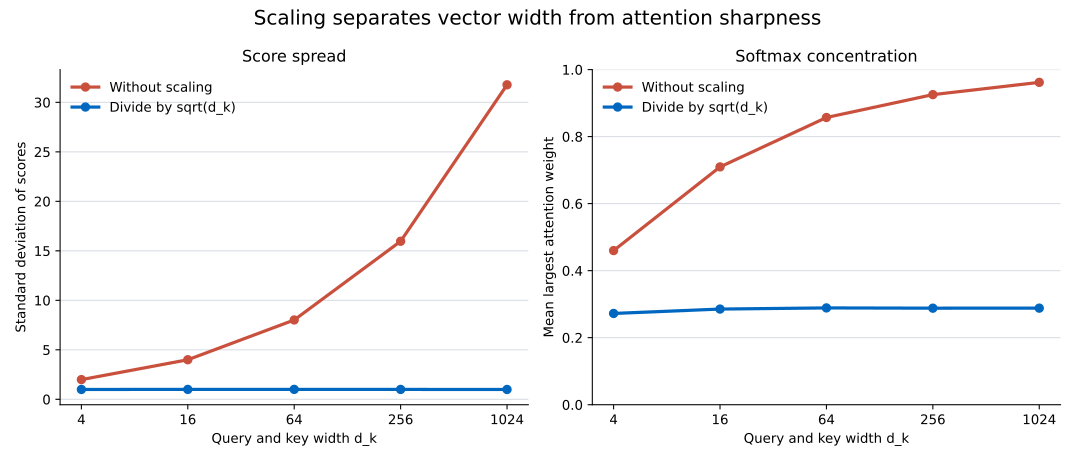
The left chart tests the variance prediction. The right chart shows the downstream softmax effect. The two blue lines stay nearly flat because scaling separates vector width from score spread. This does not mean real attention weights must stay flat as a model learns; training can change the query and key distributions.

Check concentration with a second measure

The largest weight is easy to read, but it reports only one key. Entropy summarizes how distributed the whole row is. A high value means weight is spread across several keys. A low value means most weight sits on a small number of keys.

For 12 keys, a perfectly uniform row has entropy log(12), or about 2.485 nats. A row with all weight on one key has entropy 0. A nat is the entropy unit produced when the calculation uses the natural logarithm.

Add this function and two metrics to simulate_width after calculating the weights:

def entropy(weights):
    return -(weights * np.log(weights)).sum(axis=-1)

mean_entropy_raw = entropy(raw_weights).mean()
mean_entropy_scaled = entropy(scaled_weights).mean()
raw_rows_over_90_pct = (raw_weights.max(axis=1) > 0.90).mean() * 100
scaled_rows_over_90_pct = (scaled_weights.max(axis=1) > 0.90).mean() * 100

The complete executed build produced these values for the narrowest and widest cases:

width  raw entropy  scaled entropy  raw rows >90%  scaled rows >90%
    4        1.575           2.121            4.0%              0.2%
 1024        0.092           2.093           88.1%              0.0%

Unscaled entropy falls close to zero at width 1,024, and 88.1% of rows give one random key more than 90% of the weight. Scaled entropy is almost unchanged, and none of the 4,000 widest scaled rows crosses 90%. Both measures support the same conclusion.

Do not turn those exact percentages into a general promise. They depend on 12 keys, standard-normal independent components, the fixed seed, and the chosen widths. The stable result is the mechanism: summing more comparable random products increases raw score spread, while dividing by sqrt(d_k) compensates for that increase.

Common mistakes and troubleshooting

Dividing by d_k instead of sqrt(d_k). The raw score variance grows like d_k, but its standard deviation grows like sqrt(d_k). Softmax receives scores, so the goal here is to stabilize their standard deviation. Dividing by the full width would make scores shrink as width grows.

Using the sequence length as d_k. d_k is the final width of each query and key vector. It is not the number of tokens or keys. In an array shaped (batch, heads, tokens, width), use the last dimension.

Scaling after softmax. Divide the scores before normalization. Dividing weights afterward makes their sum less than 1 and does not undo softmax concentration.

Calling np.exp on large raw scores. A direct softmax can overflow even when the final mathematical weights are valid. Subtract the maximum score in each row before exponentiation. Scaling and stable softmax solve different problems, so use both.

Forgetting the row axis. Attention normalizes the key scores for each query separately. Use axis=-1 and keepdims=True in the teaching function. Check that every output row sums to 1.

Expecting scaling to make weights uniform. It only removes predictable width-driven growth. A trained model can and should create sharp attention when its learned queries and keys support that result.

Treating the simulation assumptions as facts about every model. Learned query and key components are not guaranteed to be independent or standard normal. The experiment explains the design rule under a clean reference case. Inspect real score distributions when diagnosing a trained model.

Comparing runs with a missing seed. Random output changes on each run without a seed. Pass an integer to default_rng and record package versions. NumPy does not promise that every random bit stream stays identical across all future versions, so save result data when exact reproduction matters.

Recap: keep width out of attention sharpness

A dot product adds one query-key product per vector position. When those products are independent and have comparable variance, the raw score variance grows with d_k, and its standard deviation grows with sqrt(d_k). Wider vectors can therefore make softmax sharp even when no key is deliberately more relevant.

The executed NumPy experiment made that effect visible. From width 4 to 1,024, unscaled score spread grew from 1.990 to 31.774, while the average largest weight grew from 0.460 to 0.962. Dividing by sqrt(d_k) kept score spread near 1 and the average largest weight near 0.28.

Keep the order clear: calculate the QKᵀ scores, divide by sqrt(d_k), apply any mask, run stable softmax, and then mix the values. Scaling does not choose what deserves attention. It prevents vector width from making that choice by itself.