How to Handle Missing Values in XGBoost Without Imputation

A broken sensor can leave an empty cell in an otherwise useful row. Deleting every incomplete row throws away the temperature, time, and equipment information that still exists. Filling every gap with one typical value also makes a modeling choice that may hide why the value is absent.

To train XGBoost with missing numeric values, keep them as NumPy or pandas NaN, pass the numeric feature table to a tree-based XGBRegressor, and call fit() as usual. Its default missing marker is NaN, and each split learns which branch receives missing rows. Split the data first, then compare this route with train-only imputation on untouched test data.

This tutorial tests that workflow on fictional cold-storage readings. You will fit XGBoost directly on incomplete features, compare it with two median-filling pipelines, and learn what the model can and cannot infer from a gap. If train/test splits and regression metrics are new to you, start with your first machine learning model.

Setup, prerequisites, and reproducible data

You should be able to run a Python script or notebook cell and recognize rows and columns in a table. You do not need to know decision-tree mathematics. We will define the missing-value terms before using them.

Create a virtual environment, activate it, and install the five libraries used in the lesson:

python -m venv .venv
source .venv/bin/activate
python -m pip install numpy pandas scikit-learn xgboost matplotlib

On Windows PowerShell, use .venv\Scripts\Activate.ps1 for the activation step. The published build ran with Python 3.13.2, NumPy 2.5.1, pandas 3.0.3, scikit-learn 1.9.0, XGBoost 3.3.0, and Matplotlib 3.11.0.

The lesson uses cold_storage_energy.csv. It is an original synthetic dataset released as CC0-1.0. All 2,400 reading IDs, measurements, gaps, and energy targets are fictional. A fixed NumPy seed of 2718 makes the build repeatable.

Each row describes one cold-storage observation. The target, cooling_energy_kwh, is the cooling energy used in kilowatt-hours. The six model features describe outdoor temperature, hour, door-open time, pallet load, humidity, and compressor age.

Load the CSV and check its size:

import pandas as pd

data = pd.read_csv(
    "https://datatweets.com/datasets/blog/xgboost-missing-values-without-imputation/cold_storage_energy.csv"
)
print(data.shape)

(2400, 8)

There are eight columns because the file also contains a readable ID and the target. Now count the gaps in every model input and in the target:

features = [
    "outside_temp_c",
    "hour",
    "door_open_minutes",
    "pallet_load_kg",
    "humidity_pct",
    "compressor_age_months",
]
target = "cooling_energy_kwh"

print(data[features + [target]].isna().sum())

outside_temp_c             0
hour                       0
door_open_minutes        369
pallet_load_kg           221
humidity_pct             299
compressor_age_months      0
cooling_energy_kwh         0
dtype: int64

Three feature columns are incomplete. The target has no gaps, so every row still has an answer from which the model can learn. A missing target is a different problem: there is no known outcome for supervised training, so XGBoost cannot use that row as a labeled example.

Inspect the gaps before modeling

A total count is useful, but it does not show what an incomplete row looks like. Display only rows with at least one missing feature, then keep a small set of columns that can be checked by eye:

incomplete = data.loc[data[features].isna().any(axis=1), [
    "reading_id",
    "door_open_minutes",
    "pallet_load_kg",
    "humidity_pct",
    "cooling_energy_kwh",
]]
print(incomplete.head().to_string(index=False))

reading_id  door_open_minutes  pallet_load_kg  humidity_pct  cooling_energy_kwh
   CS-0002                6.9             NaN          69.5               50.29
   CS-0006                NaN          1352.9          62.0               61.40
   CS-0012                NaN           833.6          46.0               65.41
   CS-0013                NaN           688.6          66.7               71.69
   CS-0015                NaN           351.5          62.9               64.63

CS-0002 has no pallet-load measurement, but it still has a door time, humidity, and target. The next four rows lack a door time, yet their other measurements remain available. Direct missing-value handling preserves those useful parts of each row.

Before choosing any method, ask why each value can be absent. A random file-transfer problem differs from a sensor that fails under high heat. Also ask whether the same cause will exist when the model receives new rows. A training-time pattern is not useful if the data collection system changes before prediction.

The percentages provide a monitoring baseline. Door-open time is absent in 15.4% of rows, humidity in 12.5%, and pallet load in 9.2%. If a future batch has 70% missing door times, it no longer resembles this training data. That change deserves investigation even if predict() still returns numbers.

Finally, distinguish a valid zero from a missing value. A recorded door-open time of 0.0 says that the door stayed closed. NaN says the system does not know the duration. Replacing one with the other changes the meaning of the row.

The mental model: a gap becomes a branch choice

NaN means “Not a Number.” In pandas and NumPy, it is the usual marker for a missing numeric value. Imputation means replacing that marker with an estimated or fixed value, such as the column median.

A tree-based XGBoost model does not need that replacement first. A decision tree repeatedly asks questions such as outside_temp_c < 26.5. For each split, XGBoost also chooses a default branch for rows whose value is missing. It learns that direction from the training data, and another split can learn a different default direction.

The official XGBoost missing-value guidance says that tree algorithms learn branch directions for missing values during training. The current XGBRegressor API uses NaN as its default missing marker.

This process is routing, not recovery. If door_open_minutes is absent, the model does not discover whether the real value was 3 or 12 minutes. It only learns which available branch tends to reduce training error for rows with that gap.

That distinction matters because absence can carry information. In this synthetic dataset, a backup controller does not record door-open time and also consumes more energy. Missing door time is therefore a useful clue. Humidity and pallet-load gaps are inserted independently, so they carry less direct information about the target.

Split before any model learns from the data

Keep 25% of the rows for a final test. A test set is a group of labeled rows that the model does not use during fitting. It estimates how the completed workflow behaves on unseen data.

The split must happen before an imputer calculates a median. Otherwise, the median would include information from the test rows. This small leak can make an evaluation look better than the workflow that will receive truly new data.

from sklearn.model_selection import train_test_split

X = data[features]
y = data[target]

X_train, X_test, y_train, y_test = train_test_split(
    X,
    y,
    test_size=0.25,
    random_state=2718,
)

print(len(X_train), len(X_test))

1800 600

The model receives 1,800 rows for learning. The same 600 test rows will grade all three missing-value routes, which makes the comparison consistent.

Random splitting is suitable for these independent fictional observations. It would not always be suitable for readings ordered over time. If your production task predicts future energy from past data, train on earlier timestamps and test on later timestamps. The split should copy the real direction of prediction.

There is another boundary to protect: decide which columns are available at prediction time. A feature recorded after the energy target would leak the answer even if the code splits rows correctly. Missing-value support does not repair an invalid feature design.

Fit XGBoost directly on NaN values

First, create a tree-based regressor. The hist tree method groups possible split values into bins for efficient training. The fixed random state and single worker make this lesson’s run reproducible.

from xgboost import XGBRegressor

def new_regressor():
    return XGBRegressor(
        objective="reg:squarederror",
        n_estimators=280,
        learning_rate=0.05,
        max_depth=4,
        min_child_weight=4,
        subsample=0.9,
        colsample_bytree=0.9,
        reg_lambda=1.0,
        tree_method="hist",
        random_state=2718,
        n_jobs=1,
    )

n_estimators is the number of boosted trees. learning_rate controls the size of each tree’s correction, and max_depth limits how many split levels one tree can contain. These are fixed here so that the preprocessing route is the main difference between models.

Fit the model on the DataFrame as it is. There is no call to fillna, dropna, or an imputer:

from sklearn.metrics import mean_absolute_error, root_mean_squared_error

native_model = new_regressor()
native_model.fit(X_train, y_train)

native_prediction = native_model.predict(X_test)
print(f"test MAE:  {mean_absolute_error(y_test, native_prediction):.3f} kWh")
print(f"test RMSE: {root_mean_squared_error(y_test, native_prediction):.3f} kWh")

test MAE:  2.493 kWh
test RMSE: 3.164 kWh

Mean absolute error (MAE) is the average absolute distance between a prediction and the real target. Root mean squared error (RMSE) also measures error in kilowatt-hours, but it gives larger misses more weight. Lower is better for both.

The successful fit shows that feature NaN values do not stop this tree model. Its average absolute test error is 2.493 kWh on this synthetic dataset. That number is not evidence about a real cooling system, and it does not yet show whether direct handling is better than filling the gaps.

You can also send a missing feature at prediction time. The two rows below are otherwise identical:

import numpy as np

scenario = pd.DataFrame([
    {
        "outside_temp_c": 30.0, "hour": 14,
        "door_open_minutes": 4.0, "pallet_load_kg": 700.0,
        "humidity_pct": 60.0, "compressor_age_months": 72,
    },
    {
        "outside_temp_c": 30.0, "hour": 14,
        "door_open_minutes": np.nan, "pallet_load_kg": 700.0,
        "humidity_pct": 60.0, "compressor_age_months": 72,
    },
])

print(native_model.predict(scenario).round(2))

[62.37 73.13]

In this fitted model, the second estimate is higher. That result is consistent with the training rows, where a missing door time is associated with backup-controller use and higher energy consumption. It does not prove that removing a sensor reading causes energy use to rise.

Compare direct handling with two imputation routes

Direct handling is a good starting point, but it should still compete against reasonable alternatives. The first alternative replaces each gap with that feature’s training median. The second adds a binary indicator for each incomplete feature: 1 means the original value was missing, and 0 means it was present.

The median is the middle non-missing value after sorting a feature. It is less affected by extreme values than the mean, which makes it a common simple choice for numeric data. However, every missing row receives the same median. Two unknown door times become identical at that feature even when their real, unseen durations differed.

An indicator keeps a second piece of information: whether the value was originally absent. The model receives both a filled numeric value and a new zero-or-one column. This route makes the missing pattern explicit, while direct XGBoost handling lets each tree split learn how to route it.

Put each SimpleImputer inside a scikit-learn Pipeline. A pipeline fits the imputer only when the complete workflow receives X_train, then applies the stored training medians to X_test. The official SimpleImputer documentation defines both the median strategy and add_indicator=True behavior.

from sklearn.impute import SimpleImputer
from sklearn.pipeline import Pipeline

median_model = Pipeline([
    ("imputer", SimpleImputer(strategy="median")),
    ("model", new_regressor()),
])

indicator_model = Pipeline([
    ("imputer", SimpleImputer(strategy="median", add_indicator=True)),
    ("model", new_regressor()),
])

The median pipeline learns these six values from the 1,800 training rows:

median_model.fit(X_train, y_train)
learned_medians = pd.Series(
    median_model.named_steps["imputer"].statistics_,
    index=features,
)
print(learned_medians)

outside_temp_c             23.90
hour                       12.00
door_open_minutes           5.00
pallet_load_kg            649.70
humidity_pct               60.75
compressor_age_months      61.00
dtype: float64

Only three of those values are used to fill gaps because the other three features are complete. The output is still worth inspecting: it confirms the unit and scale of each stored statistic. When the pipeline later sees X_test, it reuses these values rather than recalculating them from test data.

Fit both pipelines and compare them with direct NaN handling on the same test targets:

models = {
    "XGBoost with NaN": native_model,
    "Median fill": median_model,
    "Median + indicators": indicator_model,
}

rows = []
for name, model in models.items():
    model.fit(X_train, y_train)
    prediction = model.predict(X_test)
    rows.append({
        "method": name,
        "mae_kwh": mean_absolute_error(y_test, prediction),
        "rmse_kwh": root_mean_squared_error(y_test, prediction),
    })

comparison = pd.DataFrame(rows)
print(comparison.round(3).to_string(index=False))

             method  mae_kwh  rmse_kwh
   XGBoost with NaN    2.493     3.164
        Median fill    2.613     3.413
Median + indicators    2.519     3.214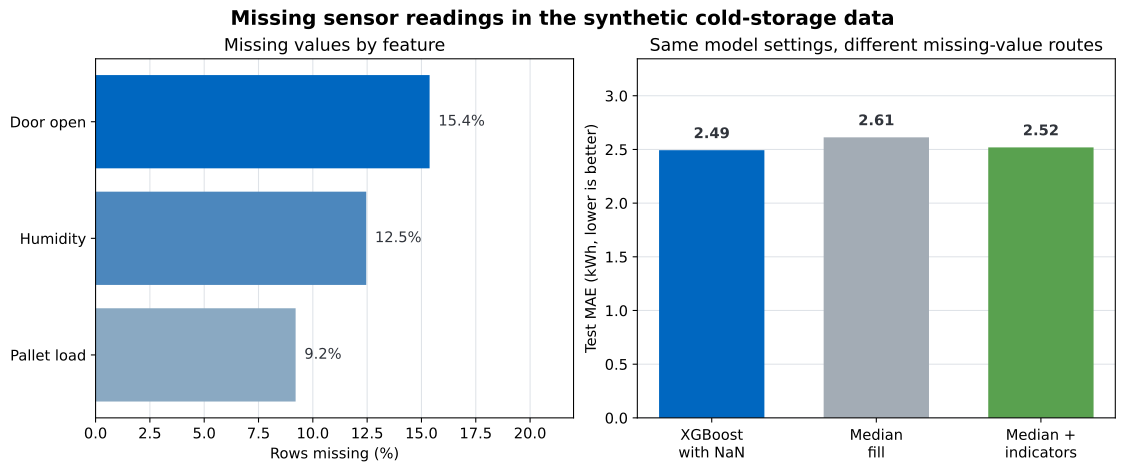

Direct handling has the lowest MAE and RMSE in this run. Plain median filling has the highest errors; it replaces missing door times with an ordinary value, so the model can no longer distinguish those gaps from recorded median values. Adding indicators preserves that distinction and narrows the error gap in this test.

The direct model’s MAE is about 0.12 kWh lower than plain median filling. That is a modest difference, not a dramatic victory. RMSE tells the same general story, which reduces the chance that the conclusion depends on only one metric. Still, these 600 test rows are one sample from a synthetic process.

The comparison controls several important choices. Every route uses the same train and test rows, the same six source features, the same XGBoost settings, and the same error functions. Only the treatment of missing values changes; the indicator route derives extra binary columns from the same source features. Without those controls, a lower score could come from a different tree depth, a different split, or extra source information rather than the missing-value method itself.

Do not turn this result into a universal rule. The three methods are close, and a different missing process can change their order. Compare routes with the same split or cross-validation plan, then prefer the simplest route whose evaluation supports it.

For a real project, repeat the comparison across several validation folds or several time periods. Also report the variation between results, not only the best average. If the methods are effectively tied, direct NaN handling removes a preprocessing step and may be easier to maintain. If an imputation route wins consistently, use the evidence rather than the shorter code.

Choose a route that matches the data process

Use direct XGBoost handling when the predictors are numeric, missing values arrive as NaN, and a tree model already fits the problem. It is especially practical when preserving incomplete rows matters. Record the missing rate for every feature so that later batches can be compared with training.

Use imputation when other parts of the workflow require complete values. For example, a separate linear model may need the same feature table. Keep the imputer inside a pipeline, and consider an indicator when the reason for absence may affect the target. Test whether that extra column helps instead of adding it automatically.

Delete rows only when the missing fields make the example unusable or when a documented data rule requires complete records. Check how many rows and which groups the deletion removes. Removing mostly one device type or operating condition can change the population that the model learns.

Whichever route you choose, save the feature list, missing marker, fitted preprocessing objects, model version, and evaluation plan together. Prediction code must apply the same meaning to gaps as training code. A model trained with NaN should not later receive an unexplained mixture of blank strings, zeros, and numeric sentinels.

Common mistakes and troubleshooting

Dropping every incomplete row. data.dropna() would remove many valid targets and complete measurements. Delete a row only when your analysis has a reason to require every selected value. If you need a broader cleaning workflow, see cleaning messy data with pandas.

Expecting XGBoost to recover the unknown value. A learned default branch is not an imputed sensor reading. Do not export it as if the model had reconstructed the missing measurement.

Calculating medians before the split. Fit preprocessing on training data only. A Pipeline makes this rule easier to preserve during testing and cross-validation.

Using a number such as -999 without declaring it. The default missing marker is NaN. If your file uses a numeric sentinel, convert it to NaN or set the model’s missing parameter deliberately. Make sure -999 cannot be a real measurement.

Confusing sparse zeros with real zeros. XGBoost’s FAQ warns that absent entries in sparse matrices can be treated as missing by tree boosters, while zero in a dense table is a valid number. Check the data representation when predictions differ after a sparse-to-dense conversion.

Assuming every XGBoost booster uses the same rule. This tutorial uses boosted trees. The linear booster treats missing values as zeros, so the learned-branch explanation does not apply to it.

Ignoring a changing missing pattern. A model can depend on the fact that a specific sensor usually fails under specific conditions. If new hardware changes that pattern, predictions can drift even when the non-missing values look familiar. Monitor missing rates by feature after deployment.

Getting different numbers. Confirm the dataset, package versions, split seed, and model settings. Keep n_jobs=1 for the closest reproduction. Floating-point details can still create small differences across platforms or later library versions.

Recap

A tree-based XGBoost regressor can fit numeric features that contain NaN. At each split, it learns a default direction for missing rows. That keeps incomplete rows available, but it does not estimate the value that was never observed.

The reliable workflow is simple: preserve missing numeric features as NaN, split the data, fit the tree model, and evaluate it on untouched rows. Then compare it with train-only imputation when the choice matters.

On this synthetic cold-storage dataset, direct handling produced 2.493 kWh test MAE. Median filling produced 2.613 kWh, while median filling plus indicators reached 2.519 kWh. The durable lesson is not the small numerical win. It is to treat missingness as a modeling signal that must be tested, documented, and monitored.