How to Build Prediction Intervals with XGBoost in Python

A batch scheduler that reports “331 seconds” hides an important difference. One job may finish within a narrow range around that estimate, while another may have a much less certain runtime because the queue is busy. A single prediction cannot show that difference.

To build prediction intervals with XGBoost, fit XGBRegressor with objective="reg:quantileerror" and quantiles such as 0.10, 0.50, and 0.90. Use the first and last predictions as a nominal 80% interval, check their order and coverage on untouched rows, then use a separate calibration set to adjust the width without consulting the final test outcomes.

This tutorial applies that workflow to fictional batch jobs. You will predict a lower runtime, a median runtime, and an upper runtime for each job. You will also see why the words “80% interval” describe a target to test, not a promise about every future job. If the basic fit-and-predict workflow is new to you, start with your first machine learning model.

Setup, prerequisites, and runtime data

You should be able to run a Python script or notebook cell and recognize rows and columns in a table. You do not need previous knowledge of quantiles, gradient boosting, or uncertainty statistics. Each term is defined when it appears.

Create a virtual environment, activate it, and install the five libraries used in the executed lesson:

python -m venv .venv
source .venv/bin/activate
python -m pip install numpy pandas scikit-learn xgboost matplotlib

On Windows PowerShell, activate the environment with .venv\Scripts\Activate.ps1. The results below were executed with Python 3.13.2, NumPy 2.5.1, pandas 3.0.3, scikit-learn 1.9.0, XGBoost 3.3.0, and Matplotlib 3.11.0.

The lesson uses batch_job_runtimes.csv. It contains 3,000 original synthetic rows released under CC0-1.0. A fixed NumPy seed generated every job ID, resource setting, queue condition, and runtime. The data is fictional and does not measure a real compute service.

Load the CSV and display five rows. The plotting backend is set to Agg before importing pyplot, so later chart code can save an SVG without a desktop window:

import math

import matplotlib

matplotlib.use("Agg")

import matplotlib.pyplot as plt
import numpy as np
import pandas as pd
from sklearn.metrics import mean_absolute_error
from sklearn.model_selection import train_test_split
from xgboost import XGBRegressor

jobs = pd.read_csv(
    "https://datatweets.com/datasets/blog/"
    "xgboost-prediction-intervals-python/batch_job_runtimes.csv"
)

print(jobs.shape)
print(jobs.head().to_string(index=False))

The executed output is:

(3000, 7)
  job_id  input_gb  cpu_cores  queue_depth  cache_hit  compression_ratio  runtime_seconds
JOB-0001     38.43          4           20          1               3.63           416.38
JOB-0002     16.33          4           10          1               3.87           195.84
JOB-0003     36.56          2           12          0               1.67           511.98
JOB-0004     19.52          4            6          0               2.80           223.32
JOB-0005      2.71          8            8          1               2.94            71.28

Each row describes one completed batch job. The target is runtime_seconds. The five model features describe input size, allocated CPU cores, queue depth, whether reusable data was found in a cache, and the compression ratio. cache_hit is an indicator: 1 means yes, and 0 means no.

The generator deliberately makes runtime variation larger for bigger inputs and deeper queues. This changing variation is called heteroscedasticity. The name is less important than the practical effect: one fixed margin such as “prediction ± 30 seconds” will not suit every row.

How a three-quantile interval works

A quantile is a boundary in an ordered set of possible outcomes. About 10% of comparable outcomes fall at or below the 10th quantile, and about 90% fall at or below the 90th quantile. The 50th quantile is the median, or middle value.

For one job, we will ask the model for these three values:

10th quantile       50th quantile       90th quantile
lower estimate  <  predicted median  <  upper estimate

The space from the 10th to the 90th quantile is a nominal 80% prediction interval because 0.90 - 0.10 = 0.80. “Nominal” means intended or labeled. We still need to measure empirical coverage: the fraction of actual test runtimes that fall between the predicted bounds.

Coverage and width must be read together. A range from 0 to one million seconds would cover almost every job, but it would not help a scheduler. A useful interval should be narrow enough to guide a decision while reaching its coverage target on relevant unseen data.

Quantile regression learns each boundary from the features. It does not take one ordinary prediction and add a constant margin. A heavy-queue job can therefore receive a wider range than a light-queue job.

Give training, calibration, and testing different jobs

Three data parts keep the evaluation honest. The training set fits XGBoost. The calibration set measures how far actual values fall outside the raw ranges and determines one shared width adjustment. The test set checks the completed procedure once.

Name the features and target explicitly, then make the two fixed splits:

FEATURES = [
    "input_gb",
    "cpu_cores",
    "queue_depth",
    "cache_hit",
    "compression_ratio",
]
TARGET = "runtime_seconds"

development, test = train_test_split(
    jobs,
    test_size=450,
    random_state=63,
)
train, calibration = train_test_split(
    development,
    test_size=450,
    random_state=63,
)

print(len(train), len(calibration), len(test))

2100 450 450

The 2,100 training rows can influence the fitted trees. The 450 calibration rows can influence the interval adjustment, but not the trees. The final 450 rows influence neither. Reusing test outcomes to choose the adjustment would turn the test set into another calibration set.

This random split is appropriate for independent fictional jobs from one stable process. For jobs ordered over time, split by time instead: older rows for training, later rows for calibration, and the newest rows for testing. That order better copies a future deployment.

Fit three quantiles in one model

XGBoost uses an objective to define the error that its trees try to reduce. reg:quantileerror uses quantile, or pinball, loss. The quantile_alpha list tells it which quantiles to estimate.

Create one regressor for the three requested quantiles. The histogram tree method is set explicitly because the official XGBoost quantile regression example uses hist and warns against the exact tree method for this objective:

QUANTILES = np.array([0.10, 0.50, 0.90])

model = XGBRegressor(
    objective="reg:quantileerror",
    quantile_alpha=QUANTILES,
    tree_method="hist",
    n_estimators=600,
    learning_rate=0.035,
    max_depth=5,
    min_child_weight=6,
    subsample=0.95,
    colsample_bytree=1.0,
    reg_lambda=2.0,
    random_state=20_260_718,
    n_jobs=1,
)

model.fit(train[FEATURES], train[TARGET])
test_predictions = model.predict(test[FEATURES])
print(test_predictions.shape)

(450, 3)

There is one row per test job and one column per requested quantile. Because QUANTILES is in ascending order, column 0 corresponds to the lower estimate, column 1 to the median, and column 2 to the upper estimate.

The number of trees, learning rate, and depth were fixed before the final test. They are teaching settings for this synthetic dataset, not universal XGBoost defaults. In a real project, tune them with training and validation data while keeping the final test separate.

Check the raw interval before trusting its label

Quantiles are estimated, so estimates for different levels can appear in the wrong order. For example, an estimated 10th quantile may be slightly above the estimated median. This is quantile crossing. XGBoost’s official example notes that crossing can happen because of an algorithm limitation.

Count crossing rows before applying a guard. Then sort each row so the first value is no greater than the second, and the second is no greater than the third:

calibration_predictions = model.predict(calibration[FEATURES])

crossing_rows = (
    (test_predictions[:, 0] > test_predictions[:, 1])
    | (test_predictions[:, 1] > test_predictions[:, 2])
).sum()
print("crossing rows:", crossing_rows)

calibration_predictions = np.sort(calibration_predictions, axis=1)
test_predictions = np.sort(test_predictions, axis=1)

crossing rows: 14

Sorting is an explicit guard that keeps the lower, middle, and upper values ordered for the calculations below. It can change which value is treated as the median, and it does not fix why the estimates crossed. A high crossing rate would be a reason to revisit the data, settings, or modeling method instead of silently sorting everything.

Now measure the raw interval. Coverage counts rows inside the bounds. Width measures the average distance from the lower to the upper estimate:

def interval_metrics(actual, lower, upper):
    actual_values = actual.to_numpy()
    covered = (actual_values >= lower) & (actual_values <= upper)
    return covered.mean(), np.mean(upper - lower)

raw_lower = test_predictions[:, 0]
median_prediction = test_predictions[:, 1]
raw_upper = test_predictions[:, 2]

raw_coverage, raw_width = interval_metrics(
    test[TARGET], raw_lower, raw_upper
)
median_mae = mean_absolute_error(test[TARGET], median_prediction)

print(f"median MAE: {median_mae:.2f} seconds")
print(f"raw coverage: {raw_coverage:.3f}")
print(f"raw average width: {raw_width:.2f} seconds")

median MAE: 19.94 seconds
raw coverage: 0.700
raw average width: 54.93 seconds

Mean absolute error (MAE) is the average absolute distance between the median prediction and the actual runtime. The median misses by 19.94 seconds on average in this test.

The more important interval result is disappointing: only 70.0% of actual runtimes fall inside a range labeled 80%. Calling the raw bounds reliable 80% intervals would overstate the executed evidence.

Widen the interval with held-out calibration errors

The calibration set tells us how far actual runtimes fall outside their raw bounds. For each calibration row, assign a nonconformity score of zero when the runtime is already inside. Otherwise, record the distance below the lower bound or above the upper bound. A larger score means the raw interval missed by more.

Calculate those scores without touching the test targets:

calibration_actual = calibration[TARGET].to_numpy()
calibration_scores = np.maximum.reduce([
    calibration_predictions[:, 0] - calibration_actual,
    calibration_actual - calibration_predictions[:, 2],
    np.zeros(len(calibration)),
])

For a target coverage of 0.80, use the finite-sample corrected position used in split conformal calibration. NumPy’s quantile documentation defines method="higher", which selects an observed score rather than interpolating between two scores:

TARGET_COVERAGE = 0.80
corrected_level = math.ceil(
    (len(calibration) + 1) * TARGET_COVERAGE
) / len(calibration)

adjustment = np.quantile(
    calibration_scores,
    corrected_level,
    method="higher",
)

calibrated_lower = raw_lower - adjustment
calibrated_upper = raw_upper + adjustment

coverage, width = interval_metrics(
    test[TARGET], calibrated_lower, calibrated_upper
)

print(f"adjustment: {adjustment:.2f} seconds")
print(f"test coverage: {coverage:.3f}")
print(f"average width: {width:.2f} seconds")

adjustment: 7.84 seconds
test coverage: 0.824
average width: 70.61 seconds

The calibration step subtracts 7.84 seconds from every lower estimate and adds 7.84 seconds to every upper estimate. In this run, test coverage rises from 70.0% to 82.4%, while average width grows from 54.93 to 70.61 seconds. The higher coverage comes with wider ranges.

The calibration targets marginal coverage, meaning coverage averaged across rows drawn from a similar process. The test set then estimates whether the completed procedure reached that target in this sample. Neither result says that every individual job has exactly an 80% chance of landing inside its range. The method also depends on training, calibration, and future jobs being comparable; a changed scheduler or hardware fleet can break that assumption.

Look beyond the overall coverage number

An overall rate can hide a weak operating region. Group the final test rows by queue depth and calculate coverage separately. These thresholds were defined as part of the fictional scenario, not chosen after seeing which group looked best:

queue_band = pd.cut(
    test["queue_depth"],
    bins=[-1, 12, 24, np.inf],
    labels=["Light (0–12)", "Busy (13–24)", "Heavy (25+)"]
)

for band in queue_band.cat.categories:
    mask = (queue_band == band).to_numpy()
    band_coverage, band_width = interval_metrics(
        test.loc[mask, TARGET],
        calibrated_lower[mask],
        calibrated_upper[mask],
    )
    print(
        f"{band}: rows={mask.sum()}, "
        f"coverage={band_coverage:.3f}, width={band_width:.2f}"
    )

Light (0–12): rows=193, coverage=0.870, width=62.67
Busy (13–24): rows=229, coverage=0.799, width=75.61
Heavy (25+): rows=28, coverage=0.714, width=84.50

The ranges become wider as the queue gets busier, which matches the synthetic data design. Yet the 28 heavy-queue jobs have only 71.4% coverage. Their small count also makes that estimate uncertain. The overall 82.4% result is therefore not enough evidence to claim good heavy-queue behavior.

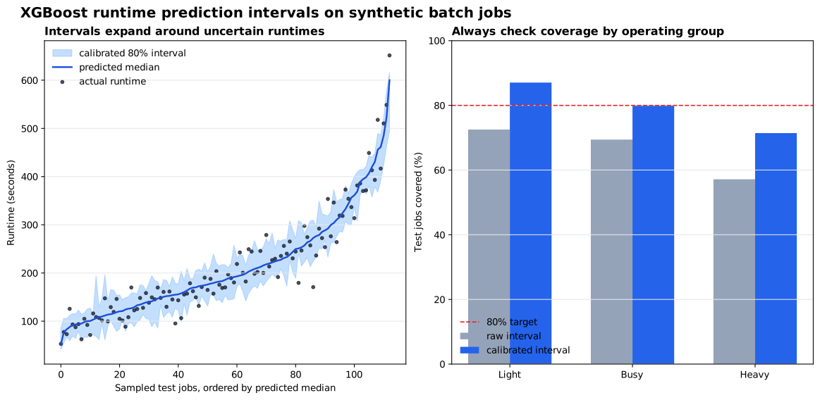
The left chart shows sampled test jobs ordered by their predicted median. The blue band changes width rather than using one fixed error bar. Points outside the band are expected occasionally, but repeated misses in one operating group require investigation.

Predict a range for one new job

Once the workflow has been evaluated, pass a new row with the same five feature names and meanings. This example describes a 28 GB input running on four CPU cores with 22 jobs already in the queue and no cache hit:

new_job = pd.DataFrame([{
    "input_gb": 28.0,
    "cpu_cores": 4,
    "queue_depth": 22,
    "cache_hit": 0,
    "compression_ratio": 2.6,
}])

new_quantiles = np.sort(model.predict(new_job)[0])
new_lower = new_quantiles[0] - adjustment
new_median = new_quantiles[1]
new_upper = new_quantiles[2] + adjustment

print(
    f"{new_lower:.1f} to {new_upper:.1f} seconds "
    f"(median {new_median:.1f})"
)

275.2 to 365.0 seconds (median 330.8)

The median is about 331 seconds, but the interval is the more useful scheduling result: roughly 275 to 365 seconds, assuming new jobs resemble the synthetic training process. It is not a service guarantee. If this range controlled real capacity, you would also monitor coverage after actual runtimes arrive.

Common mistakes and a final recap

If reg:quantileerror is unknown, check the installed XGBoost version. The current XGBoost parameter reference records that this objective was added in version 2.0.0. Upgrade in your virtual environment instead of changing the objective name.

If predictions have shape (rows,) rather than (rows, 3), confirm that quantile_alpha received a NumPy array or list with three values. Also confirm their intended order before labeling columns.

Do not calibrate on training predictions. A model often looks unusually accurate on rows used to fit its trees, so their miss distances can produce an adjustment that is too small. Do not calibrate on the final test set either; that removes your independent check.

Never assume that overall coverage applies to every subgroup. Monitor the groups that affect decisions, but avoid making strong claims from tiny groups. Collect more heavy-queue examples here before relying on that part of the range.

Finally, remember the durable workflow:

1. Choose lower and upper quantiles whose difference matches the intended coverage.
2. Keep training, calibration, and test rows separate.
3. Check output shape and quantile crossing.
4. Measure both interval coverage and width on untouched data.
5. Inspect important operating groups and monitor them after deployment.

XGBoost supplies the conditional quantile estimates. Calibration and evaluation supply the evidence needed to turn those estimates into a useful interval. If your next dataset contains missing numeric features, XGBoost can also learn missing-value branches without imputation, but the same rule still applies: test the completed workflow on data that did not fit it.